Particle swarm optimization: Difference between revisions
m (Updated PSO flow diagram) |
m (Added doi link to reference 17) |
||
| (2 intermediate revisions by the same user not shown) | |||
| Line 35: | Line 35: | ||
==Algorithm Discussion== | ==Algorithm Discussion== | ||
The structure of the algorithm is simple. The algorithm seeks to find an optimum of an objective function, <math> f(x) </math>. A set of particles, <math> X </math> with members <math> x \in X </math>, forming a swarm, is initialized randomly. The algorithm runs for a number of iterations. At each iteration, for each particle in the swarm, each particle’s position is updated to be <math> x_{ i+1, p} = x_{i, p} + v_{i, p} </math>. Subscript <math> i </math> indicates the iteration of the algorithm. Subscript <math> p </math> indicates the index of the particle in the swarm. Both the optimal solution for a particular particle, <math> x_{best, p} </math>, and a global optimum, <math> x_{best, g} </math> are tracked. <math> f(x_{best, p}) </math> is the best solution to the objective function that a particular particle, <math> p </math>, has experienced over all iterations. <math> f(x_{best, g}) </math> is the best solution to the objective function for all particles, at all iterations. The algorithm is halted when either a fixed number of iterations is reached or a stopping criteria is reached. A typical stopping criteria is when the change between iterations is below a user-set threshold, demonstrating that the particles are not moving from the identified solution point. The algorithm’s control flow is shown in the following flow chart. | The structure of the algorithm is simple. The algorithm seeks to find an optimum of an objective function, <math> f(x) </math>. A set of particles, <math> X </math> with members <math> x \in X </math>, forming a swarm, is initialized randomly. The algorithm runs for a number of iterations. At each iteration, for each particle in the swarm, each particle’s position is updated to be <math> x_{ i+1, p} = x_{i, p} + v_{i, p} </math>. Subscript <math> i </math> indicates the iteration of the algorithm. Subscript <math> p </math> indicates the index of the particle in the swarm. Both the optimal solution for a particular particle, <math> x_{best, p} </math>, and a global optimum, <math> x_{best, g} </math> are tracked. <math> f(x_{best, p}) </math> is the best solution to the objective function that a particular particle, <math> p </math>, has experienced over all iterations. <math> f(x_{best, g}) </math> is the best solution to the objective function for all particles, at all iterations. The algorithm is halted when either a fixed number of iterations is reached or a stopping criteria is reached. A typical stopping criteria is when the change between iterations is below a user-set threshold, demonstrating that the particles are not moving from the identified solution point. The algorithm’s control flow is shown in the following flow chart. | ||
[[File:PSO Flow.png|center|frameless | |||
[[File:PSO Algorithm Flow.png|400px|center|frameless|Particle Swarm Optimization Algorithm Flow Chart]] | |||
<div style="text-align:center;font-size:1em;"> | <div style="text-align:center;font-size:1em;"> | ||
Figure 1: Algorithm Flow Chart | Figure 1: Algorithm Flow Chart | ||
| Line 173: | Line 175: | ||
===Step 3: Define Stopping Criteria === | ===Step 3: Define Stopping Criteria === | ||
For this example | For this example select a maximum number of iterations (t): | ||
<div style="text-align:center;font-size:1em;"> | <div style="text-align:center;font-size:1em;"> | ||
| Line 257: | Line 259: | ||
Objective Function: <math> f(x,y) = sin(5x+1)+cos(7y-3)+x^2+y^2 \,</math> | Objective Function: <math> f(x,y) = sin(5x+1)+cos(7y-3)+x^2+y^2 \,</math> | ||
From Step 2, | From Step 2, the defined number of particles is <math> P = 25 \,</math> | ||
| Line 268: | Line 270: | ||
For each particle, determine the best value in its own history. This will be called "Personal Best Objective Function" and notated as <math> pbo^i \,</math>. At initialization, there is only one value. | For each particle, determine the best value in its own history. This will be called "Personal Best Objective Function" and notated as <math> pbo^i \,</math>. At initialization, there is only one value. | ||
In effect | In effect the program is tracking the position and value of each particle through all iterations and choosing the optimal value - in this example the minimum. As such, rather than tracking all values, the computational memory needs can be reduced by only tracking the optima found so far and comparing to the next iteration’s value: | ||
| Line 478: | Line 480: | ||
<ref> Gudise, V.G. and Venayagamoorthy, G.K. (2003) Comparison of particle swarm optimization and backpropagation as training algorithms for neural networks, ''Proceedings of the 2003 IEEE Swarm Intelligence Symposium'', (pp.110-117) doi: 10.1109/SIS.2003.1202255</ref>. | <ref> Gudise, V.G. and Venayagamoorthy, G.K. (2003) Comparison of particle swarm optimization and backpropagation as training algorithms for neural networks, ''Proceedings of the 2003 IEEE Swarm Intelligence Symposium'', (pp.110-117) doi: 10.1109/SIS.2003.1202255</ref>. | ||
However, the current state of the current practice for training deep neural networks remains the back-propagation algorithm. Back-propagation is more efficient in the context of neural networks because for each particle at each iteration, there will need to be an error function computation. For example, a swarm size of 25 requires 25 times more error function evaluations | However, the current state of the current practice for training deep neural networks remains the back-propagation algorithm. Back-propagation is more efficient in the context of neural networks because for each particle at each iteration, there will need to be an error function computation. For example, a swarm size of 25 requires 25 times more error function evaluations | ||
<ref name=wihartiko> Wihartiko, F. (2018) Performance comparison of gentitic algorithms and particle swarm optimization for model integer programming bus timetabling problem, ''IOP Conference Series: Materials Science and Engineering'' doi:10.1088/1757-899X/332/1/012020 </ref>. | <ref name=wihartiko> Wihartiko, F. (2018) Performance comparison of gentitic algorithms and particle swarm optimization for model integer programming bus timetabling problem, ''IOP Conference Series: Materials Science and Engineering'', doi:10.1088/1757-899X/332/1/012020 </ref>. | ||
In addition to identifying weights in the Neural Networks (training), PSO has been used in selecting hyperparameters for neural networks. In these applications PSO is used to maximize the neural network’s accuracy by varying parameters including number of nodes and structure of the networks | In addition to identifying weights in the Neural Networks (training), PSO has been used in selecting hyperparameters for neural networks. In these applications PSO is used to maximize the neural network’s accuracy by varying parameters including number of nodes and structure of the networks | ||
<ref> Lorenzo, Pablo et al (2017) Particle swarm optimization for hyperparameter selection in deep neural networks, | <ref> Lorenzo, Pablo et al (2017) Particle swarm optimization for hyperparameter selection in deep neural networks, ''Proceedings of the Genetic and Evolutionary Computation Conference (pp. 481-488) https://doi.org/10.1145/3071178.3071208</ref>. | ||
PSO fits this application well because this function is nonlinear and the gradient is non-continuous. Hyperparameters for NNs may be real, integer or binary values. | PSO fits this application well because this function is nonlinear and the gradient is non-continuous. Hyperparameters for NNs may be real, integer or binary values. | ||
| Line 492: | Line 494: | ||
Pymoo is an alternative Python implementation | Pymoo is an alternative Python implementation | ||
<ref name=pymoo/>. | <ref name=pymoo/>. | ||
Pyswarms is a compact implementation specifically focused on PSO, whereas Pymoo is a more complete library with multiple | Pyswarms is a compact implementation specifically focused on PSO, whereas Pymoo is a more complete library with multiple optimization algorithm implementations. Matlab does have PSO implementation as part of the optimization toolbox | ||
<ref> MathWorks (2024) particleswarm, Retrieved 2024 from https://www.mathworks.com/help/gads/particleswarm.html </ref> | <ref> MathWorks (2024) particleswarm, Retrieved 2024 from https://www.mathworks.com/help/gads/particleswarm.html </ref> | ||
There is a 3rd party Matlab implementation available for free | There is a 3rd party Matlab implementation available for free | ||
Revision as of 12:22, 14 December 2024
Author: David Schluneker (dms565), Thomas Ploetz (tep52), Michael Sorensen (mds385), Amrith Kumaar (ak836), Andrew Duffy (ajd296) (ChemE 6800 Fall 2024)
Stewards: Nathan Preuss, Wei-Han Chen, Tianqi Xiao, Guoqing Hu
Introduction
Particle Swarm Optimization (PSO) is inspired by nature and groups or swarms of natural creatures. It uses multiple “particles” distributed across a solution space to slowly converge upon a global, optimized solution. This algorithm does not require calculation of the function’s gradient or slope, instead using simple weights and the contribution of the rest of the swarm to provide a “fitness” value [1] to leading to a technique dependent only on simple calculations and a number of starting points.
The PSO algorithm was formulated and initially presented by Kennedy and Eberhart specifically to find solutions to discontinuous, but non-differentiable functions. The concept was presented at the IEEE conference on neural networks in 1995 [2]. The pair later published a book Swarm Intelligence in 2001 that further expanded on the concept [3]. Others have summarized the algorithm [4] [5] [6]. This algorithm does not leverage formal methodology or mathematical rigor to identify an ideal point but instead uses a heuristic approach to explore a wide range of starting locations and conditions. These features allow the PSO algorithm to efficiently optimize complex functions.
The biological analogy for a PSO algorithm is a flock of birds, a school of fish, or a colony of ants trying to find a food resource. Each animal, or particle, is an independent entity that is conducting its own search routine for an optimal result. However, the particles will also be influenced and guided by motions of the larger swarm. The results any particle has already seen, as well as the influence of the larger swarm helps all the particles converge to an optimal solution.
In a more technical dissection, a PSO algorithm must be initially set-up with how many particles and iterations the user wants to use. More particles improve the convergence likelihood and help ensure the global optimum can be found due to a more complete search at the cost of computing resources required. The PSO algorithm allows a user to set different “weights”, step sizes, and speeds for the particles to control how influenced each particle is by its past points (cognitive) and by the other nearby points (social) in the swarm and how large of steps will be taken. These weights allow algorithm adjustment to tailor the performance and computational requirements.
The goals of studying this topic are to learn more about an algorithm capable of solving nondifferentiable functions that are relevant to modern problems. Many optimization algorithms use the gradient function, so it is interesting to see an algorithm that does not require gradient computations. Additionally, the algorithm is still in active use in many fields [6] [7]. PSO is regularly used to solve optimization problems in the gas and oil industry, antenna design [8], and electric power distribution [9]. As functions get very complex in the real-world, the PSO algorithm is still capable of performing an effective search within very complex functions due to its heuristic and operability on non-differentiable functions.
Algorithm Discussion
The structure of the algorithm is simple. The algorithm seeks to find an optimum of an objective function, . A set of particles, with members , forming a swarm, is initialized randomly. The algorithm runs for a number of iterations. At each iteration, for each particle in the swarm, each particle’s position is updated to be . Subscript indicates the iteration of the algorithm. Subscript indicates the index of the particle in the swarm. Both the optimal solution for a particular particle, , and a global optimum, are tracked. is the best solution to the objective function that a particular particle, , has experienced over all iterations. is the best solution to the objective function for all particles, at all iterations. The algorithm is halted when either a fixed number of iterations is reached or a stopping criteria is reached. A typical stopping criteria is when the change between iterations is below a user-set threshold, demonstrating that the particles are not moving from the identified solution point. The algorithm’s control flow is shown in the following flow chart.
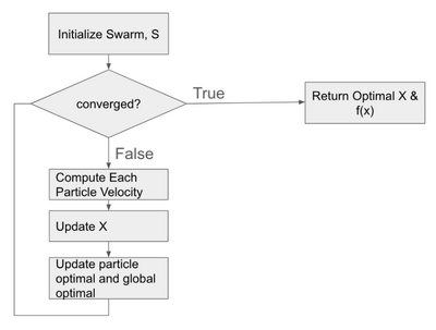
Figure 1: Algorithm Flow Chart
A velocity, is independently computed for each particle . The velocity is the result of the sum of the preceding velocity, a cognitive component and a social component. The cognitive component is and pulls the solution towards the best point observed by this particle. The social component is and pulls the solution towards the best point observed across the entire swarm. Each of the social component and cognitive component are weighed by a factor. The state that must be tracked across loop iterations is; , , for each particle and .
The convergence of the algorithm can be checked in a few different ways. The original papers were based on training neural networks, so the optimization was halted when the neural network was sufficiently able to make predictions [2] [10]. This approach is flawed because the designer of the algorithm used a priori knowledge of how good the neural network will perform. More generally, this approach incorporates application specific logic to stop when the optimal solution is good enough. Alternatively, the algorithm can be terminated following a predetermined number of iterations. Another approach is to stop when the solution's improvement at a given iteration stops [11].
The pseudocode for the PSO algorithm attempting to minimize a solution follows. The algorithm can be modified to search for a maximum by changing the initialization of and along with their updates.
SWARM is initialized randomly
initialized to 0
initialized to
initialized to
For i in MAX_ITERATIONS:
For particle in SWARM:
if
if
PRINT “Local optimal at ”
Figure 2: Algorithm Pseudocode
The algorithm has a few hyperparameters including; number of particles in the swarm, weights of the cognitive update on the velocity, weights on the social update on the velocity. The Pymoo Python implementation suggests a swarm size of 25, velocity weight of 0.8, a social update weight of 2.0 and a cognitive update of 2.0 [12]. Practitioners will need to adjust parameters and determine how their problem reacts to modifications of the hyperparameters. Heuristics may be used to adjust the various weights between iterations of the algorithm. Algorithms that adjust the hyperparameters based on heuristics are called Adaptive Particle Swarm Optimization (APSO) [13].
PSO makes very few assumptions. The algorithm can be trivially adopted to work with real, integer or mixed functions. The algorithm does not rely on gradients or hessians, so there are no assumptions or requirements on the function being continuous or differentiable. However, the lack of assumptions comes at a cost, there is no proof that the algorithm will find an optimal solution. One of the original papers by Kennedy in 1997 [10] indicated a tendency for the optimization to get stuck in local minimum. Adjustment of the algorithm’s hyperparameters is a performance vs robustness trade that may have avoided sticking in a local optimum.
Numerical Example
This section will walk through a numerical example of solving a complex objective function using Particle Swarm Optimization.
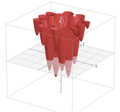
Given a non-convex function with multiple local optima:
Step 1: Define the Objective Function
Objective Function:
Step 2: Define Key Variables
| Symbol | Description | Value | Additional Notes |
|---|---|---|---|
| P | Total Number of Particles used to search the function | 25 | Larger number means greater chance of finding the global optimum, but larger computational load |
| random number between 0 and 1 | (0,1) | to be randomly generated at each evaluation | |
| random number between 0 and 1 | (0,1) | to be randomly generated at each evaluation | |
| Inertia Weight Constant (0,1) | 0.7 | ||
| Cognitive Coefficient
(Independence, prioritize the self) |
0.1* | recommend & sufficiently low value for slower smoother operation | |
| Social Coefficient
(Codependence, prioritize the group) |
0.15* | recommend & sufficiently low value for slower smoother operation |
- The algorithm is highly sensitive to c1 and c2. Recommend referencing the search space and using 1/30 to 1/60 of the total range. Ex: target search range is -3 to 3 by -3 to 3, use a value 0.1 to 0.2 to prevent “overshooting” and oscillations of the individual particles.
Step 3: Define Stopping Criteria
For this example select a maximum number of iterations (t):
It is important to note that there are alternative stopping criteria such as checking for convergence of the particles - such as a minimum delta between points or using a Confidence Interval on the X and Y coordinates as your threshold. This could lead to more, or less, iterations depending upon what threshold is used. Care should be taken to ensure the stopping criteria can actually be met. This wiki does not provide an example of this methodology at this point in time.
Step 4: Setup Particle Data
Each particle has three main properties
- Position of particle , at iteration , denoted as where:
or
- Velocity Vector denoted as:
or
- Objective Function Value of:
Where equals total number of particles, cumulatively these would be represented as:
This wiki uses not due to starting at not
Important Note only tracks the current iteration of particle , not all values of a particle over iterations:
and and
This wiki guide will use randomly generated initialization for particle position and velocity. There are alternative initialization methods available that are not covered in this guide such as using a set of points in a grid pattern.
For and , define initialization data for all particles given and define a range to search within:
To ensure an even distribution and less initial clustering of the particles, this example will use a uniform distribution to create surrogate data to initialize the position. Depending on how the code is set up, scaling and offset factors may be required.
This example will use a normal distribution to create surrogate data to initialize the Velocity vector. Depending how the code is set up, a scaling factor may be required.
Example Particle Data, Particle # 7:
- Particle Position Coordinates at time () :
- Particle Velocity Vector at time () :
- Particle Objective Value at time () :
Step 5: Evaluate Function at Positions
For each particle, evaluate the objective function at their position:
Objective Function:
From Step 2, the defined number of particles is
Step 5.1 - Calculate Local Optima
For each particle, determine the best value in its own history. This will be called "Personal Best Objective Function" and notated as . At initialization, there is only one value.
In effect the program is tracking the position and value of each particle through all iterations and choosing the optimal value - in this example the minimum. As such, rather than tracking all values, the computational memory needs can be reduced by only tracking the optima found so far and comparing to the next iteration’s value:
Note: becomes in the next iteration.
Cumulatively this can also be written as:
Note: Shown is at . All "best" values occur at upon initialization.
The location of the optimal objective function value () at () needs to be recorded. () will be used to notate the "Personal Best Location" or the positional coordinates that return the best () ever explored by particle () .
Cumulatively written as:
Step 5.2 - Calculate Global Optima
Now that the personal best for all particles is known, the next step is to compare all particles to determine the best global value. The "Global Best Objective Function Value" will be notated as , this represent the best explored by all particles.
correlates to or particle 12 of 24 (25 particles = particle 0 , ... particle 24 )
The Global Best Objective Function Value was determined in the previous step, next the coordinates that achieved that value needs to be recorded. "Global Best Location" is notated as to represent the position that gives the best explored by all particles.
Step 6: Calculate Next Iteration Position, Velocity, Value
Calculate the next iteration values by using the following rules:
Position:
Velocity:
Note: need to generate a random value for and at this step
Example:
Determine where :
Requires determining first:
Define Variables:
Solve for :
Solve for :
Reevaluate :
Step 7: Iteratively Solve
Calculate next optima, position, velocity, and function values for each particle. Repeat until stopping criteria has been met.
Final Results after iterations:
Global Best Value: :
Global Best Position: :
Visual Representation
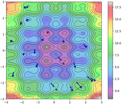
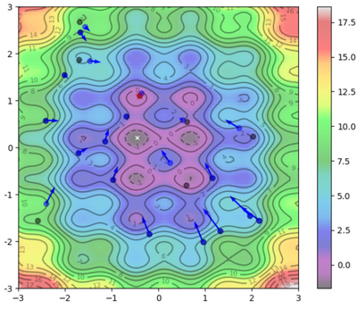
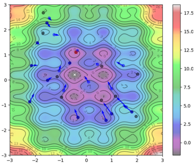
To help visualize what's going on:
Blue Dots = Each particle's current position
Blue Arrows = Each particle's velocity
Black Dots = Each particle's best position
| Iteration | Image |
|---|---|
| |
| |
| |
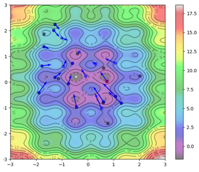
| |
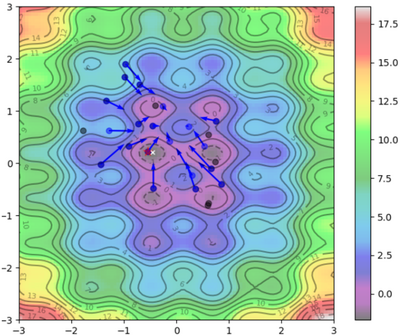
| |
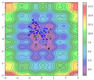
| |
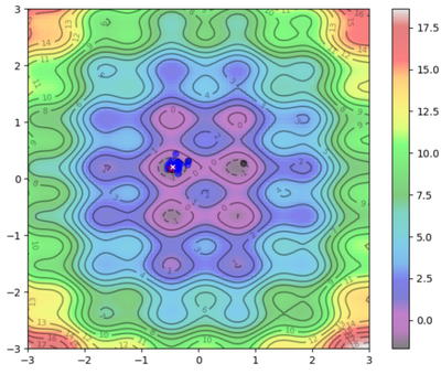
|
Applications
The strength of PSO is in its simplicity and ability to handle arbitrary functions. The algorithm does not use gradient information, making it useful in contexts where computation of the gradient is expensive or the function is otherwise unreliable.
PSO was originally used to train neural networks (NN)[2]. Neural networks frequently have highly non-linear loss functions and it is therefore difficult to find a global optimum [14]. Several papers have noted an improvement in NN accuracy using PSO optimization when compared to back-propagation due to the ability to avoid local optimum [15]. However, the current state of the current practice for training deep neural networks remains the back-propagation algorithm. Back-propagation is more efficient in the context of neural networks because for each particle at each iteration, there will need to be an error function computation. For example, a swarm size of 25 requires 25 times more error function evaluations [16].
In addition to identifying weights in the Neural Networks (training), PSO has been used in selecting hyperparameters for neural networks. In these applications PSO is used to maximize the neural network’s accuracy by varying parameters including number of nodes and structure of the networks [17]. PSO fits this application well because this function is nonlinear and the gradient is non-continuous. Hyperparameters for NNs may be real, integer or binary values.
PSO is most often compared to other heuristic based algorithms such as; genetic algorithms differential evolution simulated annealing. One study for a bus scheduling application did find the PSO was better than genetic algorithms with respect to the optimality of solution and run-time [16]. The results in the paper are difficult to generalize, as results will be sensitive to the application as well as the algorithm’s hyperparameters. The recommended choice of heuristic optimization algorithms remains up to the practitioner’s judgement.
A number of different implementations are available as libraries. Pyswarms is a Python API [18] Pymoo is an alternative Python implementation [12]. Pyswarms is a compact implementation specifically focused on PSO, whereas Pymoo is a more complete library with multiple optimization algorithm implementations. Matlab does have PSO implementation as part of the optimization toolbox [19] There is a 3rd party Matlab implementation available for free [20]. However, the algorithm is simple so many prefer to implement the algorithm directly.
Conclusions
The PSO algorithm is a heuristic based optimization algorithm. The heuristics are loosely based on the behavior of a flock of seagulls. The algorithm’s strengths are in its simplicity, lack of reliance on a gradient, and robustness against getting stuck in local optimum. The drawback is that the “swarm” requires a large number of function evaluations, making the algorithm slow. Additionally, the algorithm has no guarantee of convergence. The ability to find an optimum is sensitive to starting conditions and hyperparameters.
The algorithm is easy to get up and running with several public implementations available in the Python and Matlab programming languages. Alternatively, the algorithm is so simple that some will implement the algorithm themselves.
When using the algorithm, practitioners need to select several weights that control the algorithms. A cognitive weight determines to what extent a particle’s previous optimum affects future searches. A social weight determines to what extent all particle’s global optimum affects future searches. These parameters and the swarm size need to be adjusted carefully to balance robustness against computational efficiency.
The PSO algorithm continues to be developed. There is research into how to adjust the algorithm’s hyperparameters at various iterations of the algorithm. These algorithms are called adaptive particle swarm optimization (APSO) and take some guesswork the algorithm. The algorithm has also been combined with genetic optimization algorithms, though the algorithms remain heuristic based and do not guarantee optimum results.
PSO continues to be used in applications that are non-linear or are non-differentiable. Recent (2024) studies have used PSO for RF in optimizing the placement of terminals [21] and for predicting landslides [22].
References
- ↑ Vyas, Ajay Kumar (2022) Artificial Intelligence for Renewable Energy Systems, John Wiley & Sons
- ↑ 2.0 2.1 2.2 Kennedy, J. and Eberhart, R. (1995) Particle Swarm Optimization, Proceedings of the IEEE International Conference on Neural Networks, (pp. 1942-1945), doi: 10.1109/ICNN.1995.488968
- ↑ Kennedy, J. and Eberhart, R. (2001) Swarm Intelligence 1st ed., Academic Press
- ↑ Rao, Singiresu (2020) Engineering Optimization - Theory and Practice (5th Edition), John Wiley and Sons
- ↑ Belyadi, Hoss and Haghighat, Alizera (2021) Machine Learning Guides for Oil and Gas Using Python - A Step-by-Step Breakdown with Data, Algorithms, Codes, and Applications, Elsevier
- ↑ 6.0 6.1 Hassan, Rania (2004) Particle Swarm Optimization: Methods and Applications, Retrieved 2024 from https://dspace.mit.edu/bitstream/handle/1721.1/68163/16-888-spring-2004/contents/lecture-notes/l13_msdo_pso.pdf
- ↑ Poli, Richard (2008) Analysis of the Publications on the Applications of Particle Swarm Optimization, Journal of Artificial Evolution and Applications (pp. 685175-685185), doi: https://doi.org/10.1155/2008/685175
- ↑ Jin, Nanbo and Rahmet-Samii, Yahya (2008) Particle Swarm Optimization for Antenna Designs in Engineering Electromagnetics, Journal of Artificial Evolution and Applications (pp. 728929-728939), doi: https://doi.org/10.1155/2008/728929
- ↑ Sharmeela, C. et al (2022) IoT, Machine Learning and Blockchain Technologies for Renewable Energy and Modern Hybrid Power Systems, River Publishers
- ↑ 10.0 10.1 Kennedy, J. (1997) The Particle Swarm: Social Adaptation of Knowledge, Proceedings of the IEEE International Conference on Evolutionary Computation (pp. 303-308), doi: 10.1109/ICEC.1997.592326
- ↑ MathWorks (2024) Particle Swarm Options, Retrieved 2024 from https://www.mathworks.com/help/gads/particle-swarm-options.html
- ↑ 12.0 12.1 Blank, Justin (2020) Multi-Objective Optimization in Python, Retrieved 2024 from https://pymoo.org/algorithms/soo/pso.html
- ↑ Zhan, Z. et al (2009) Adaptive Particle Swarm Optimization, IEEE Transactions on Systems, Man, and Cybernetics, Part B (Cybernetics), vol. 39, no. 6, (pp.1362-1381) doi: 10.1109/TSMCB.2009.2015956
- ↑ Want, C. et al (2024) cuPSO: GPU Parallelization for Particle Swarm Optimization Algorithms, arXiv:2205.01313v2, Retrieved 2024 from https://arxiv.org/pdf/2205.01313
- ↑ Gudise, V.G. and Venayagamoorthy, G.K. (2003) Comparison of particle swarm optimization and backpropagation as training algorithms for neural networks, Proceedings of the 2003 IEEE Swarm Intelligence Symposium, (pp.110-117) doi: 10.1109/SIS.2003.1202255
- ↑ 16.0 16.1 Wihartiko, F. (2018) Performance comparison of gentitic algorithms and particle swarm optimization for model integer programming bus timetabling problem, IOP Conference Series: Materials Science and Engineering, doi:10.1088/1757-899X/332/1/012020
- ↑ Lorenzo, Pablo et al (2017) Particle swarm optimization for hyperparameter selection in deep neural networks, Proceedings of the Genetic and Evolutionary Computation Conference (pp. 481-488) https://doi.org/10.1145/3071178.3071208
- ↑ James, Lester (2017) PySwarms, Retrieved 2024 from https://pyswarms.readthedocs.io/en/latest/
- ↑ MathWorks (2024) particleswarm, Retrieved 2024 from https://www.mathworks.com/help/gads/particleswarm.html
- ↑ Birge, Brian (2024) Particle Swarm Optimization Toolbox, https://www.mathworks.com/matlabcentral/fileexchange/7506-particle-swarm-optimization-toolbox, MATLAB Central File Exchange.
- ↑ Urbanus Mwanzia Ngei, et al (2024) Optimal sizing and placement of STATCOM, TCSC and UPFC using a novel hybrid genetic algorithm-improved particle swarm optimization, Heliyon vol. 10, issue 23, https://doi.org/10.1016/j.heliyon.2024.e40682
- ↑ Zhang, Qing (2024) Spatial distribution prediction of landslide susceptibility based on integrated particle swarm optimization, Frontiers in Earth Science vol. 12, doi=10.3389/feart.2024.1516615




![{\displaystyle X^{i}(t)=[X^{0}(t),\cdots ,X^{P-1}(t)]={\begin{bmatrix}x^{0}(t),&\cdots ,&x^{P-1}(t)\\y^{0}(t),&\cdots ,&y^{P-1}(t)\end{bmatrix}}}](https://wikimedia.org/api/rest_v1/media/math/render/svg/0b4cc2f97269944129e5de0095d2381396424965)
![{\displaystyle V^{i}(t)=[V^{0}(t),\cdots ,V^{P-1}(t)]={\begin{bmatrix}V_{x}^{0}(t),&\cdots ,&V_{x}^{P-1}(t)\\V_{y}^{0}(t),&\cdots ,&V_{y}^{P-1}(t)\end{bmatrix}}}](https://wikimedia.org/api/rest_v1/media/math/render/svg/5069ed09a314fc4e558fcc4df3b0f5f93db3d828)
)]=[f(x^{0}(t),y^{0}(t)),\cdots ,f(x^{P-1}(t),y^{P-1}(t))\,}](https://wikimedia.org/api/rest_v1/media/math/render/svg/a5c0802c6b060df904e71c6846dc4cc1e189621a)


![{\displaystyle f(X^{7}(t))\neq [f(x^{7}(0),y^{7}(0),\cdots ,f(x^{7}(m),y^{7}(m)]}](https://wikimedia.org/api/rest_v1/media/math/render/svg/7aa7afb4e9059e6409d27482be739f7cc809104e)


![{\displaystyle pbo^{i}=min[f^{i}(X^{i}(0)),\cdots ,f^{i}(X^{i}(m))]\rightarrow min[f^{i}(X^{i}(t_{previousbest}^{i})),f^{i}(X^{i}(t))]=[f^{i}(X^{i}(t_{best}^{i}))]\,}](https://wikimedia.org/api/rest_v1/media/math/render/svg/69b0f04ff4f12f5b09fdb661057f2837e5292556)


![{\displaystyle pbo=[min[f^{0}(X^{0}(t_{previousbest}^{0})),f^{0}(X^{0}(t))],\cdots ,min[f^{P-1}(X^{P-1}(t_{previousbest}^{P-1})),f^{P-1}(X^{P-1}(t))]]=\,}](https://wikimedia.org/api/rest_v1/media/math/render/svg/733826e148e123873028c967d7894b27a69654de)
![{\displaystyle pbo=[f^{0}(X^{0}(t_{b}est^{0})),\cdots ,f^{P-1}(X^{P-1}(t_{best}^{P-1}))]=\,}](https://wikimedia.org/api/rest_v1/media/math/render/svg/55a72227f6ac42d117c64209cdf1d5e0ce8c5df1)
![{\displaystyle pbo=[-1.6941,\cdots ,-1.7126]\,}](https://wikimedia.org/api/rest_v1/media/math/render/svg/7765481af2cdca3544d3ef8da296d243b1d1fee8)


![{\displaystyle pb^{i}=[X^{i}(0),\cdots ,X^{i}(m)]\rightarrow [X^{i}(t_{best}^{i})]={\begin{bmatrix}x^{i}(t_{best}^{i})\\y^{i}(t_{best}^{i})\end{bmatrix}}\,}](https://wikimedia.org/api/rest_v1/media/math/render/svg/511e8df2710ea78fa3125d0551c6827799b24168)
![{\displaystyle pb=[X^{0}(t_{best}^{0}),\cdots ,X^{P-1}(t_{best}^{P-1})]={\begin{bmatrix}x^{0}(t_{best}^{0}),&\cdots ,&x^{P-1}(t_{best}^{P-1})\\y^{0}(t_{best}^{0}),&\cdots ,&y^{P-1}(t_{best}^{P-1})\end{bmatrix}}\,}](https://wikimedia.org/api/rest_v1/media/math/render/svg/b0f9309c1e60b53db13690af62370b616406b2f8)

![{\displaystyle gbo=min[pbo]=f(X(t_{best}))}](https://wikimedia.org/api/rest_v1/media/math/render/svg/18538d2d0be2b42e065611fc60e9e5b41f454cb8)
![{\displaystyle gbo=min[-1.6941,\cdots ,-1.7126]}](https://wikimedia.org/api/rest_v1/media/math/render/svg/ca2ff2e011afa9f41f93204e99bbdf9a0b6d7ba7)
![{\displaystyle gbo=[-1.7137]}](https://wikimedia.org/api/rest_v1/media/math/render/svg/8a88e6b5dfc02db731c1df65c2064fdadd30bdc9)


![{\displaystyle gb=[X(t_{best})]}](https://wikimedia.org/api/rest_v1/media/math/render/svg/b7805bb09945a12e727b3d64f3e18e46e8a8592a)
![{\displaystyle gb=pb^{12}=[X^{12}(t_{best}^{12})]={\begin{bmatrix}x^{12}(t_{best}^{12})\\y^{12}(t_{best}^{12})\end{bmatrix}}={\begin{bmatrix}-0.4832\\0.1907\end{bmatrix}}}](https://wikimedia.org/api/rest_v1/media/math/render/svg/959221a6c5b2aa177fbb6e991d5afff9f65072b9)


