Subgradient optimization: Difference between revisions
No edit summary |
|||
| (17 intermediate revisions by the same user not shown) | |||
| Line 4: | Line 4: | ||
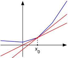
[[File:Subderivative_illustration.png|right|thumb|A convex nondifferentiable function (blue) with red "subtangent" lines generalizing the derivative at the nondifferentiable point ''x''<sub>0</sub>.]] | [[File:Subderivative_illustration.png|right|thumb|A convex nondifferentiable function (blue) with red "subtangent" lines generalizing the derivative at the nondifferentiable point ''x''<sub>0</sub>.]] | ||
The '''subgradient method''' is a simple algorithm for the optimization of non-differentiable functions, and it originated in the Soviet Union during the 1960s and 70s, primarily by the contributions of Naum Z. Shor (Sharma, Shashi). While the calculations for this approach are similar to that of the gradient method for differentiable functions, there are several key differences. First, as noted the subgradient method applies strictly to non-differentiable functions as it reduces to the gradient method when f is differentiable. Secondly the step size is fixed before the application of the algorithm rather than being determined “on-line” as in other approaches. Finally the subgradient method is not a descent method as the value of f can and often will increase. | The '''subgradient method''' is a simple algorithm for the optimization of non-differentiable functions, and it originated in the Soviet Union during the 1960s and 70s, primarily by the contributions of Naum Z. Shor (Sharma, Shashi). While the calculations for this approach are similar to that of the gradient method for differentiable functions, there are several key differences. First, as noted the subgradient method applies strictly to non-differentiable functions as it reduces to the gradient method when <math>f</math> is differentiable. Secondly the step size is fixed before the application of the algorithm rather than being determined “on-line” as in other approaches. Finally the subgradient method is not a descent method as the value of f can and often will increase. | ||
==Introduction== | ==Introduction== | ||
The subgradient method is more computationally expensive when compared to Newton's method but applicable to a wider range of problems. Additionally, due to the method’s schema when applied numerically the memory requirements are smaller than other methods allowing larger problems to be approached. Further the combination of the subgradient method with the primal dual decomposition can simplify some applications to a distributed algorithm. | The subgradient method is more computationally expensive when compared to Newton's method but applicable to a wider range of problems. Additionally, due to the method’s schema when applied numerically the memory requirements are smaller than other methods allowing larger problems to be approached. Further the combination of the subgradient method with the primal dual decomposition can simplify some applications to a distributed algorithm. | ||
==Algorithm Discussion== | ==Algorithm Discussion== | ||
'''Basics:''' | '''Basics:''' | ||
Starting with a convex function f | Starting with a convex function, <math>f</math>, such that <math>f:\mathbb{R}^n \to \mathbb{R}</math>. The classic implementation of the sub-gradient method iterates: | ||
<math>x^{(k+1)} = x^{(k)} - \alpha_k g^{(k)}</math> | <math>x^{(k+1)} = x^{(k)} - \alpha_k g^{(k)}</math> | ||
where g(k) denotes any subgradient of f at x^(k)and x^(k) is the k^th iteration of x. A subgradient of f | where <math>g(k)</math> denotes any subgradient of <math>f</math> at <math>x^{(k)}</math> and <math>x^{(k)}</math> is the <math>k^{th}</math> iteration of <math>x</math>. A subgradient of <math>f</math> is defined as: | ||
<math>g^{(k)} \in \partial f(x^{(k)})</math> | <math>g^{(k)} \in \partial f(x^{(k)})</math> | ||
In the case where | In the case where <math>f</math> is differentiable then the subgradient reduces to <math>\nabla f</math>, recovering the gradient method. It is possible that <math>-g(k)</math>is not a descent direction of <math>f</math> at <math>x^{(k)}</math>. This means that the method requires a list of the lowest objective function values found thus far <math>f_{best}</math>: | ||
<math>f^{(k)}_{\text{best}} = \min \{ f^{(k-1)}_{\text{best}}, f(x^{(k)}) \}</math> | <math>f^{(k)}_{\text{best}} = \min \{ f^{(k-1)}_{\text{best}}, f(x^{(k)}) \}</math> | ||
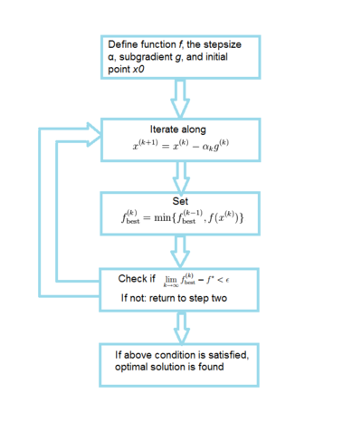
An algorithm flowchart is provided below for the subgradient method: <br/> | |||
[[File:SMFlowsheet.png|400px|center]] | |||
'''Step Size Considerations:''' | |||
The step size for this algorithm is determined externally to the algorithm itself. There are a number of methods for determining the step size:<br/> | |||
*Constant step size: | |||
**<math>\alpha_k = \alpha</math> | |||
*Constant step length: | |||
**<math>\alpha_k = \frac{\gamma}{\| g^{(k)} \|_2} \quad </math> which gives <math>\quad \| x^{(k+1)} - x^{(k)} \|_2 = \gamma</math> | |||
*Square Summable but not summable step size: | |||
**<math>\alpha_k \geq 0, \quad \sum_{k=1}^\infty \alpha_k^2 < \infty, \quad \sum_{k=1}^\infty \alpha_k = \infty</math> | |||
*Non Summable diminishing: | |||
**<math>\alpha_k \geq 0, \quad \lim_{k \to \infty} \alpha_k = 0, \quad \sum_{k=1}^\infty \alpha_k = \infty</math> | |||
*Non Summable diminishing step lengths: | |||
**<math>\gamma_k \geq 0, \quad \lim_{k \to \infty} \gamma_k = 0, \quad \sum_{k=1}^\infty \gamma_k = \infty</math> | |||
*Polyak’s Step length: | |||
**<math>\alpha_k = \frac{f(x^{(k)}) - f^*}{\| g^{(k)} \|_2^2}</math> | |||
'''Convergence:''' | '''Convergence:''' | ||
In the case of constant step-length and scaled subgradients having Euclidean norms equal to one, the method converges within an arbitrary error | In the case of constant step-length and scaled subgradients having Euclidean norms equal to one, the method converges within an arbitrary error, <math>\epsilon</math>, or: | ||
<math>\quad \lim_{k \to \infty} f^{(k)}_{\text{best}}-f*<\epsilon</math> | |||
This case however is slow and has poor performance. As such, it is largely used in specialized applications due to the simplicity and adaptability for specialized problem structures. | |||
==Numerical Example== | |||
We have a piecewise linear function: | |||
<math> \begin{align} f(x) = x < -2, -2x + 8\\ | |||
-2 \leq x \leq 4, -x + 11\\ | |||
4 \leq x \leq 7, x + 3\\ | |||
7 < x, 3x + 9\end{align} </math> | |||
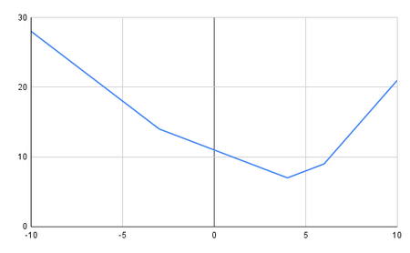
[[File:SubGradientExampleChart.png|450px|thumb|This graph illustrates the piecewise function, f(x).]] | |||
'''Table 1: Raw Data'''<br/> | |||
[[File:SubGradientExampleTable.PNG]] | |||
'''Step 1:''' Initial guess of <math>x</math> value and step size, <math>k</math> | |||
*<math>x = -9</math> and <math>k = 0.1</math> | |||
'''Step 2:''' Calculate <math>x^{(k+1)}</math> | |||
*<math>-9 - 0.1 \cdot (-2) = -8.8</math> | |||
'''Step 3:''' Evaluate <math>f(x^{(k+1)})</math> | |||
*<math>-2 \cdot x^{(k+1)} + 8 = -2 \cdot -8.8 + 8 = 25.6</math> | |||
'''Step 4:''' Store the <math>min(f_{best}, f(x^{(k+1)})</math> | |||
*<math>min(-8.8, 25.6) = -8.8</math> | |||
'''Step 5:''' Check that error against tolerance, iterate (return to Step 2) if error > <math>\epsilon</math> | |||
*<math>25.6 - 7 = 18.6 > \epsilon</math> so we return to Step 2 using <math>-8.8</math> as <math>x_k</math> | |||
*On iteration 155, <math>7 - 7 = 0 < \epsilon</math> so we have solved the problem | |||
'''Step 6:''' Optimal solution is determined | |||
== | ==Applications== | ||
Subgradient methods are generally for solving non-differentiable optimization problems. This algorithm is used in data science applications such as machine learning whenever the gradient method is not sufficient. It is also found in applications like engineering where it is utilized for problems in robotics and power systems (Licio, Romao). | Subgradient methods are generally for solving non-differentiable optimization problems. This algorithm is used in data science applications such as machine learning whenever the gradient method is not sufficient. It is also found in applications like engineering where it is utilized for problems in robotics and power systems (Licio, Romao). | ||
In some applications, the combination of the subgradient method and the primal dual decomposition can simplify to a distributed algorithm. This is shown in detail in Adaptive Subgradient Methods for Online Learning and Stochastic Optimization (Duchi et al.). The experiments outlined focus on different data sets such as text and images, and then use the subgradient method in order to flexibly be applied in various geometries. This adaptive characteristic provides unique benefits such as improved performance for identification of predictive attributes when compared to non-adaptive alternatives. | In some applications, the combination of the subgradient method and the primal dual decomposition can simplify to a distributed algorithm. This is shown in detail in Adaptive Subgradient Methods for Online Learning and Stochastic Optimization (Duchi et al.). The experiments outlined focus on different data sets such as text and images, and then use the subgradient method in order to flexibly be applied in various geometries. This adaptive characteristic provides unique benefits such as improved performance for identification of predictive attributes when compared to non-adaptive alternatives. | ||
Some commercial tools like MATLAB and optimization solvers like Gurobi, FICO, and MOSEK contain the subgradient method algorithm. There are also open-source solvers like Couenee and GLPK that support this function. Alternatively, CVXPY is an open-source Python embedded modeling language that contains subgradient methods in its library. | Some commercial tools like MATLAB and optimization solvers like Gurobi, FICO, and MOSEK contain the subgradient method algorithm. There are also open-source solvers like Couenee and GLPK that support this function. Alternatively, CVXPY is an open-source Python embedded modeling language that contains subgradient methods in its library. | ||
==Conclusion== | ==Conclusion== | ||
| Line 108: | Line 103: | ||
==References== | ==References== | ||
1. | 1. Boyd, Stephen. “Subgradient Methods.” web.stanford.edu, 2014, https://web.stanford.edu/class/ee364b/lectures/subgrad_method_notes.pdf <br/> | ||
2. | 2. Duchi, John, et al. “Adaptive Subgradient Methods for Online Learning and Stochastic Optimization.” Journal of Machine Learning Research, 11 7 2011, https://www.jmlr.org/papers/volume12/duchi11a/duchi11a.pdf <br/> | ||
3. | 3. Sharma, Shashi. “Analysis on Sub-Gradient and Semi-Definite Optimization.” Journal of Advances and Scholarly Researches in Allied Education, vol. 12, no. 2, Jan. 2017 <br/> | ||
4. | 4. Romao, Licio, et al. “Subgradient Averaging for Multi-Agent Optimisation with Different Constraint Sets.” ScienceDirect, Pergamon, 2 June 2021, www.sciencedirect.com/science/article/abs/pii/S0005109821002582 <br/> | ||
5. Shor, N. Z. "Minimization Methods for Non-differentiable Functions". Springer Series in Computational Mathematics. Springer, 1985 | 5. Shor, N. Z. "Minimization Methods for Non-differentiable Functions". Springer Series in Computational Mathematics. Springer, 1985 <br/> | ||
Latest revision as of 13:38, 15 December 2024
Author: Malichi Merski (mm2835), Ryan Ortiz (rjo64), Nicholas Phillips (ntp28) (ChemE 6800 Fall 2024)
Stewards: Nathan Preuss, Wei-Han Chen, Tianqi Xiao, Guoqing Hu

The subgradient method is a simple algorithm for the optimization of non-differentiable functions, and it originated in the Soviet Union during the 1960s and 70s, primarily by the contributions of Naum Z. Shor (Sharma, Shashi). While the calculations for this approach are similar to that of the gradient method for differentiable functions, there are several key differences. First, as noted the subgradient method applies strictly to non-differentiable functions as it reduces to the gradient method when $ f $ is differentiable. Secondly the step size is fixed before the application of the algorithm rather than being determined “on-line” as in other approaches. Finally the subgradient method is not a descent method as the value of f can and often will increase.
Introduction
The subgradient method is more computationally expensive when compared to Newton's method but applicable to a wider range of problems. Additionally, due to the method’s schema when applied numerically the memory requirements are smaller than other methods allowing larger problems to be approached. Further the combination of the subgradient method with the primal dual decomposition can simplify some applications to a distributed algorithm.
Algorithm Discussion
Basics:
Starting with a convex function, $ f $, such that $ f:\mathbb{R}^n \to \mathbb{R} $. The classic implementation of the sub-gradient method iterates:
$ x^{(k+1)} = x^{(k)} - \alpha_k g^{(k)} $
where $ g(k) $ denotes any subgradient of $ f $ at $ x^{(k)} $ and $ x^{(k)} $ is the $ k^{th} $ iteration of $ x $. A subgradient of $ f $ is defined as:
$ g^{(k)} \in \partial f(x^{(k)}) $
In the case where $ f $ is differentiable then the subgradient reduces to $ \nabla f $, recovering the gradient method. It is possible that $ -g(k) $is not a descent direction of $ f $ at $ x^{(k)} $. This means that the method requires a list of the lowest objective function values found thus far $ f_{best} $:
$ f^{(k)}_{\text{best}} = \min \{ f^{(k-1)}_{\text{best}}, f(x^{(k)}) \} $
An algorithm flowchart is provided below for the subgradient method:

Step Size Considerations:
The step size for this algorithm is determined externally to the algorithm itself. There are a number of methods for determining the step size:
- Constant step size:
- $ \alpha_k = \alpha $
- Constant step length:
- $ \alpha_k = \frac{\gamma}{\| g^{(k)} \|_2} \quad $ which gives $ \quad \| x^{(k+1)} - x^{(k)} \|_2 = \gamma $
- Square Summable but not summable step size:
- $ \alpha_k \geq 0, \quad \sum_{k=1}^\infty \alpha_k^2 < \infty, \quad \sum_{k=1}^\infty \alpha_k = \infty $
- Non Summable diminishing:
- $ \alpha_k \geq 0, \quad \lim_{k \to \infty} \alpha_k = 0, \quad \sum_{k=1}^\infty \alpha_k = \infty $
- Non Summable diminishing step lengths:
- $ \gamma_k \geq 0, \quad \lim_{k \to \infty} \gamma_k = 0, \quad \sum_{k=1}^\infty \gamma_k = \infty $
- Polyak’s Step length:
- $ \alpha_k = \frac{f(x^{(k)}) - f^*}{\| g^{(k)} \|_2^2} $
Convergence:
In the case of constant step-length and scaled subgradients having Euclidean norms equal to one, the method converges within an arbitrary error, $ \epsilon $, or: $ \quad \lim_{k \to \infty} f^{(k)}_{\text{best}}-f*<\epsilon $
This case however is slow and has poor performance. As such, it is largely used in specialized applications due to the simplicity and adaptability for specialized problem structures.
Numerical Example
We have a piecewise linear function:
$ \begin{align} f(x) = x < -2, -2x + 8\\ -2 \leq x \leq 4, -x + 11\\ 4 \leq x \leq 7, x + 3\\ 7 < x, 3x + 9\end{align} $

Step 1: Initial guess of $ x $ value and step size, $ k $
- $ x = -9 $ and $ k = 0.1 $
Step 2: Calculate $ x^{(k+1)} $
- $ -9 - 0.1 \cdot (-2) = -8.8 $
Step 3: Evaluate $ f(x^{(k+1)}) $
- $ -2 \cdot x^{(k+1)} + 8 = -2 \cdot -8.8 + 8 = 25.6 $
Step 4: Store the $ min(f_{best}, f(x^{(k+1)}) $
- $ min(-8.8, 25.6) = -8.8 $
Step 5: Check that error against tolerance, iterate (return to Step 2) if error > $ \epsilon $
- $ 25.6 - 7 = 18.6 > \epsilon $ so we return to Step 2 using $ -8.8 $ as $ x_k $
- On iteration 155, $ 7 - 7 = 0 < \epsilon $ so we have solved the problem
Step 6: Optimal solution is determined
Applications
Subgradient methods are generally for solving non-differentiable optimization problems. This algorithm is used in data science applications such as machine learning whenever the gradient method is not sufficient. It is also found in applications like engineering where it is utilized for problems in robotics and power systems (Licio, Romao).
In some applications, the combination of the subgradient method and the primal dual decomposition can simplify to a distributed algorithm. This is shown in detail in Adaptive Subgradient Methods for Online Learning and Stochastic Optimization (Duchi et al.). The experiments outlined focus on different data sets such as text and images, and then use the subgradient method in order to flexibly be applied in various geometries. This adaptive characteristic provides unique benefits such as improved performance for identification of predictive attributes when compared to non-adaptive alternatives.
Some commercial tools like MATLAB and optimization solvers like Gurobi, FICO, and MOSEK contain the subgradient method algorithm. There are also open-source solvers like Couenee and GLPK that support this function. Alternatively, CVXPY is an open-source Python embedded modeling language that contains subgradient methods in its library.
Conclusion
In summary, the subgradient method is a simple algorithm for the optimization of non-differentiable functions. While its performance is not as desirable as other algorithms, its simplicity and adaptability to problem formulation keeps it in use for a number of applications. As always, problem formulation should be a key consideration in the selection of this algorithm. A number of variations on step size and solutions exist extending the applicability of this method and it should be considered for the case of non-differentiable problems.
References
1. Boyd, Stephen. “Subgradient Methods.” web.stanford.edu, 2014, https://web.stanford.edu/class/ee364b/lectures/subgrad_method_notes.pdf
2. Duchi, John, et al. “Adaptive Subgradient Methods for Online Learning and Stochastic Optimization.” Journal of Machine Learning Research, 11 7 2011, https://www.jmlr.org/papers/volume12/duchi11a/duchi11a.pdf
3. Sharma, Shashi. “Analysis on Sub-Gradient and Semi-Definite Optimization.” Journal of Advances and Scholarly Researches in Allied Education, vol. 12, no. 2, Jan. 2017
4. Romao, Licio, et al. “Subgradient Averaging for Multi-Agent Optimisation with Different Constraint Sets.” ScienceDirect, Pergamon, 2 June 2021, www.sciencedirect.com/science/article/abs/pii/S0005109821002582
5. Shor, N. Z. "Minimization Methods for Non-differentiable Functions". Springer Series in Computational Mathematics. Springer, 1985