Network flow problem: Difference between revisions
No edit summary |
|||
| (26 intermediate revisions by 5 users not shown) | |||
| Line 1: | Line 1: | ||
Author: Aaron Wheeler, Chang Wei, Cagla Deniz Bahadir, Ruobing Shui, Ziqiu Zhang ( | Author: Aaron Wheeler, Chang Wei, Cagla Deniz Bahadir, Ruobing Shui, Ziqiu Zhang (ChemE 6800 Fall 2020) | ||
== Introduction == | == Introduction == | ||
Network flow problems arise in several key instances and applications within society and have become fundamental problems within computer science, operations research, applied mathematics, and engineering. Developments in the approach to tackle these problems resulted in algorithms that became the chief instruments for solving problems related to large-scale systems and industrial logistics. Spurred by early developments in linear programming, the methods for addressing these extensive problems date back several decades and they evolved over time as the use of digital computing became increasingly prevalent in industrial processes. Historically, the first instance of an algorithmic development for the network flow problem came in 1956, with the network simplex method formulated by George Dantzig.< | Network flow problems arise in several key instances and applications within society and have become fundamental problems within computer science, operations research, applied mathematics, and engineering. Developments in the approach to tackle these problems resulted in algorithms that became the chief instruments for solving problems related to large-scale systems and industrial logistics. Spurred by early developments in linear programming, the methods for addressing these extensive problems date back several decades and they evolved over time as the use of digital computing became increasingly prevalent in industrial processes. Historically, the first instance of an algorithmic development for the network flow problem came in 1956, with the network simplex method formulated by George Dantzig.<sup>[1]</sup> A variation of the simplex algorithm that revolutionized linear programming, this method leveraged the combinatorial structure inherent to these types of problems and demonstrated incredibly high accuracy.<sup>[2]</sup> This method and its variations would go on to define the embodiment of the algorithms and models for the various and distinct network flow problems discussed here. | ||
== Theory, Methodology, and Algorithms == | == Theory, Methodology, and Algorithms == | ||
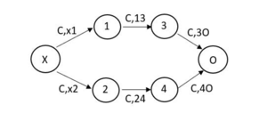
The network flow problem can be conceptualized as a directed graph which abides by flow capacity and conservation constraints. The vertices in the graph are classified into origins (source <math>X</math>), destinations (sink <math>O</math>), and intermediate points and are collectively referred to as nodes (<math>N</math>). These nodes are different from one another such that <math>N_i \neq X,O,\ldots N_j</math>.<sup>[3]</sup> The edges in the directed graph are the directional links between nodes and are referred to as arcs (<math>A</math>). These arcs are defined with a specific direction <math>(i, j)</math> that corresponds to the nodes they are connecting. The arcs <math>A\subseteq (i,j)</math> are also defined by a specific flow capacity <math>c(A)>0</math> that cannot be exceeded. The supply and demand of units <math>\Sigma_i u_i=0~for~i\in N</math> are formulated by negative and positive flow notation, and are defined such that sources equate to positive values (supply) and sinks equate to negative values (demand). Intermediate nodes have no net supply or demand. Figure 1 illustrates this general definition of the network. | |||
[[File:Picture1.png|thumb|Figure 1. General Network Flow Problem]] | |||
Additional constraints of the network flow optimization model place limits on the solution and vary significantly based on the specific type of problem being solved. Historically, the classic network flow problems are considered to be the maximum flow problem and the minimum-cost circulation problem, the assignment problem, bipartite matching problem, transportation problem, and the transshipment problem.<sup>[2]</sup> The approach to these problems become quite specific based upon the problem’s objective function but can be generalized by the following iterative approach: 1. determining the initial basic feasible solution; 2. checking the optimality conditions (i.e. whether the problem is infeasible, unbounded over the feasible region, optimal solution has been found, etc.); and 3. constructing an improved basic feasible solution if the optimal solution has not been determined.<sup>[3]</sup> | |||
=== General Applications === | === General Applications === | ||
==== The Assignment Problem ==== | ==== The Assignment Problem ==== | ||
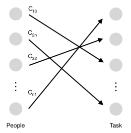
Various real-life instances of assignment problems exist for optimization, such as assigning a group of people to different tasks, events to halls with different capacities, rewards to a team of contributors, and vacation days to workers. All together, the assignment problem is a bipartite matching problem in the kernel. <sup>[3]</sup> In a classical setting, two types of objects of equal amount are bijective (i.e. they have one-to-one matching), and this tight constraint ensures a perfect matching. The objective is to minimize the cost or maximize the profit of matching, since different items of two types have distinct affinity. [[File:Assignment.png|thumb|Figure | Various real-life instances of assignment problems exist for optimization, such as assigning a group of people to different tasks, events to halls with different capacities, rewards to a team of contributors, and vacation days to workers. All together, the assignment problem is a bipartite matching problem in the kernel. <sup>[3]</sup> In a classical setting, two types of objects of equal amount are bijective (i.e. they have one-to-one matching), and this tight constraint ensures a perfect matching. The objective is to minimize the cost or maximize the profit of matching, since different items of two types have distinct affinity. [[File:Assignment.png|thumb|Figure 2. Classic model of assignment problem|alt=|267x267px]]A classic example is as follows: suppose there are <math> n </math> people (set <math> P </math>) to be assigned to <math> n </math> tasks (set <math> T </math>). Every task has to be completed and each task has to be handled by only one person, and <math> c_{ij} </math>, usually given by a table, measures the benefits gained by assigning the person <math> i </math> (in <math> P </math>) to the task <math> j </math> (in <math> T </math>). <sup>[4]</sup> The natural objective here is to maximize the overall benefits by devising the optimal assignment pattern. A graph of the general assignment problem and a table of preference are depicted as Figure 2 and Table 2. | ||
{| class="wikitable sortable" | {| class="wikitable sortable" | ||
|+Table 1. Table of preference | |+Table 1. Table of preference | ||
| Line 59: | Line 57: | ||
|3 | |3 | ||
|} | |} | ||
Figure | Figure 2 can be viewed as a network. The nodes represent people and tasks, and the edges represent potential assignments between a person and a task. Each task can be completed by any person. However, the person that actually ends up being assigned to the task will be the lone individual who is best suited to complete. In the end, the edges with positive flow values will be the only ones represented in the finalized assignment. <sup>[5]</sup> | ||
To approach this problem, the binary variable <math> x_{ij} </math> is defined as whether the person <math> i </math> is assigned to the task <math> j </math>. If so, <math> x_{ij} </math> = 1, and <math> x_{ij} </math> = 0 otherwise. | To approach this problem, the binary variable <math> x_{ij} </math> is defined as whether the person <math> i </math> is assigned to the task <math> j </math>. If so, <math> x_{ij} </math> = 1, and <math> x_{ij} </math> = 0 otherwise. | ||
| Line 91: | Line 89: | ||
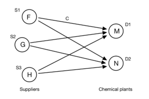
There are 2 chemical plants located in 2 different places: <math> M </math> and <math> N </math>. There are 3 raw material suppliers in other 3 locations: <math> F </math>, <math> G </math>, and <math> H </math>. The amount of materials from a supplier can be arbitrarily divided into two parts and shipped to two factories. Supplier <math> F </math>, <math> G </math>, and <math> H </math> can provide <math> S_1 </math>, <math> S_2 </math>, and <math> S_3 </math> amounts of materials respectively. The chemical plants located at <math> M </math> and <math> N </math> have the material demand of <math> D_1 </math> and <math> D_2 </math> respectively. Each transportation route, from suppliers to chemical plants, is attributed with a specific cost. This model raises the question: to keep the chemical plants running, what is the best way to arrange the material from the suppliers so that the transportation cost could be minimized? | There are 2 chemical plants located in 2 different places: <math> M </math> and <math> N </math>. There are 3 raw material suppliers in other 3 locations: <math> F </math>, <math> G </math>, and <math> H </math>. The amount of materials from a supplier can be arbitrarily divided into two parts and shipped to two factories. Supplier <math> F </math>, <math> G </math>, and <math> H </math> can provide <math> S_1 </math>, <math> S_2 </math>, and <math> S_3 </math> amounts of materials respectively. The chemical plants located at <math> M </math> and <math> N </math> have the material demand of <math> D_1 </math> and <math> D_2 </math> respectively. Each transportation route, from suppliers to chemical plants, is attributed with a specific cost. This model raises the question: to keep the chemical plants running, what is the best way to arrange the material from the suppliers so that the transportation cost could be minimized? | ||
[[File:Transportation problem example.png|thumb|Figure | [[File:Transportation problem example.png|thumb|Figure 3. Transportation problem example]] | ||
Several quantities should be defined to help formulate the frame of the solution: | Several quantities should be defined to help formulate the frame of the solution: | ||
| Line 175: | Line 173: | ||
==== The Shortest-Path Problem ==== | ==== The Shortest-Path Problem ==== | ||
The shortest-path problem can be defined as finding the path that yields the shortest total distance between the origin and the destination. Each possible stop is a node and the paths between these nodes are edges incident to these nodes, where the path distance becomes the weight of the edges. In addition to being the most common and straightforward application for finding the shortest path, this model is also used in various applications depending on the definition of nodes and edges. <sup>[3]</sup> For example, when each node represents a different object and the edge specifies the cost of replacement, the equipment replacement problem is derived. Moreover, when each node represents a different project and the edge specifies the relative priority, the model becomes a project scheduling problem. | The shortest-path problem can be defined as finding the path that yields the shortest total distance between the origin and the destination. Each possible stop is a node and the paths between these nodes are edges incident to these nodes, where the path distance becomes the weight of the edges. In addition to being the most common and straightforward application for finding the shortest path, this model is also used in various applications depending on the definition of nodes and edges. <sup>[3]</sup> For example, when each node represents a different object and the edge specifies the cost of replacement, the equipment replacement problem is derived. Moreover, when each node represents a different project and the edge specifies the relative priority, the model becomes a project scheduling problem. | ||
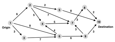
[[File:Shortest-Path.png|thumb|443x443px|Figure | [[File:Shortest-Path.png|thumb|443x443px|Figure 4. General form of shortest-path problem]] | ||
A graph of the general shortest-path problem is depicted as Figure | A graph of the general shortest-path problem is depicted as Figure 4: | ||
In the general form of the shortest-path problem, the variable <math> x_{ij} </math> represents whether the edge <math> (i,j) </math> is active (i.e. with a positive flow), and the parameter <math> c_{ij} </math> (e.g. <math> c_{12} </math> = 6) defines the distance of the edge <math> (i,j) </math>. The general problem is formulated as below: | In the general form of the shortest-path problem, the variable <math> x_{ij} </math> represents whether the edge <math> (i,j) </math> is active (i.e. with a positive flow), and the parameter <math> c_{ij} </math> (e.g. <math> c_{12} </math> = 6) defines the distance of the edge <math> (i,j) </math>. The general problem is formulated as below: | ||
| Line 199: | Line 197: | ||
Consider the following scenario: | Consider the following scenario: | ||
[[File:Picture2.png|thumb|Figure | [[File:Picture2.png|thumb|Figure 5. Maximal flow problem example]] | ||
The given structure is a piping system. The water flows into the system from the source node, passing through the intermediate nodes, and flows out from the sink node. There is no limitation on the amount of water that can be used as the input for the source node. Therefore, the sink node can accept an unlimited amount of water coming into it. The arrows denote the valid channel that water can flow through, and each channel has a known flow capacity. What is the maximum flow that the system can take? | The given structure is a piping system. The water flows into the system from the source node, passing through the intermediate nodes, and flows out from the sink node. There is no limitation on the amount of water that can be used as the input for the source node. Therefore, the sink node can accept an unlimited amount of water coming into it. The arrows denote the valid channel that water can flow through, and each channel has a known flow capacity. What is the maximum flow that the system can take? | ||
Several quantities should be defined to help formulate the frame of the solution: | Several quantities should be defined to help formulate the frame of the solution: | ||
[[File:Picture3.png|thumb|Figure | [[File:Picture3.png|thumb|Figure 6. For every intermediate node j, there is a group of node i and a group of node k.]] | ||
For any intermediate node <math display="inline">j | For any intermediate node <math display="inline">j | ||
</math> in the system, it receives water from adjacent node(s) <math>i | </math> in the system, it receives water from adjacent node(s) <math>i | ||
| Line 299: | Line 297: | ||
Using the definitions above: | Using the definitions above: | ||
[[File:Picture4.png|thumb|Figure | [[File:Picture4.png|thumb|Figure 7. The imaginary flow connects the sink node to the source node, creating a close loop.]] | ||
min<math> \quad z = \sum_k^r x_{uk} | min<math> \quad z = \sum_k^r x_{uk} | ||
| Line 331: | Line 329: | ||
=== Algorithms === | === Algorithms === | ||
==== Ford–Fulkerson Algorithm ==== | |||
A broad range of network flow problems could be reduced to the max-flow problem. The most common way to approach the max-flow problem in polynomial time is the Ford-Fulkerson Algorithm (FFA). FFA is essentially a greedy algorithm and it iteratively finds the augmenting s-t path to increase the value of flow. The pathfinding terminates until there is no s-t path present. Ultimately, the max-flow pattern in the network graph will be returned. <sup>[8]</sup> | |||
Typically, FFA is applied to flow networks with only one source node s and one sink node t. In addition, the capacity conditions and the conservation conditions, which are two properties defining the flow, must be satisfied.<sup>[9]</sup> The capacity conditions require that each edge carry a flow that is no more than its capacity, or <math>0\leq f(e)\leq c_{e},\forall e\in E</math>, where function f returns the flow on a certain edge. The conservation conditions require all nodes except the source and the sink to have a net flow of 0, or ,<math>\sum_{e~into~v}f(v)= \sum_{e~out~of~v}f(v),\forall v\in V-{s,t} </math>. | |||
FFA introduces the concept of residue graph based on the original graph <math>G</math> to allow backtracking, or pushing backward on edges that are already carrying flow.<sup>[9]</sup> The residue graph <math>G_{f} </math>is defined as the following: | |||
1. <math>G_{f}</math>has exactly the same node set as <math>G</math>. | |||
2. For each edge <math>e = (u,v)</math>with a nonnegative flow <math> f( e)</math> in <math>G</math>, <math>G_{f}</math>has the edge e with the capacity <math>c(e)_{f} = c_{e} - f(e)</math>, and also <math>G_f</math> has the edge <math>e' = (v,u)</math> with the capacity <math>c(e')_{f} = f(e)</math>. | |||
Note that initially, the <math>G_{f} </math> is identical to <math>G</math> since there is no flow present in <math>G</math>. | |||
The steps of FFA are as below. <sup>[10]</sup> Essentially, the method repeatedly finds a path with positive flow in the residue graph, and updates the flow graph and residue graph until <math>s</math> and <math>t</math> become disjoint in the residue graph. | |||
1. Set <math>f(e) = 0, \forall e\in E</math>in <math>G</math>, and create a copy as <math>G_{f}</math>. | |||
2. While there is still a <math>s, t</math> path <math>p</math> in <math>G_{f}</math>: | |||
a. Find <math>c_{f}(p) = min(c_{f}(e):e\in p)</math> | |||
b. For each edge <math>e\in p</math>: | |||
bi. <math>f(e) = f(e) + c_{f}(p)</math> if <math>e\in E</math> in <math>G</math>, <math>f(e) = f(e) - c_{f}(p)</math> if <math>e'\in E</math> in <math>G</math> | |||
bii. <math>c(e)= c(e) - c_{f}(p),c(e')= c(e') + c_{f}(p)</math> in <math> G_{f}</math> | |||
[[File:Phase 1.png|thumb|Figure 8: Flow graph and residue graph at the first phase]] | |||
An example of running the FFA is as below. | |||
The flow graph <math>G</math> and residue graph<math>G_{f}</math> at the initial phase is depicted in Figure 8, where the number of each edge in the flow graph is the flow units on the edge, whereas it is the updated edge capacity in the residue graph. | |||
In the residue graph, an <math>s-t</math> path can be found in the residue graph tracing the edge <math>s\rightarrow A\rightarrow B\rightarrow t</math> with the flow of two units. After augmenting the path on both graphs, the flow graph and the residue graph look like the Figure 9. | |||
[[File:Phase 2.png|thumb|Figure 9: Flow graph and residue graph after updating with the first s,t-path]] | |||
At this stage, there is still <math>s,t</math>-path in the residue graph <math>s\rightarrow B\rightarrow A\rightarrow t</math> with a flow of one unit. After augmenting the path on both graphs, the flow graph and the residue graph look like the Figure 10. | |||
[[File:Phase 3.png|thumb|Figure 10: Flow graph and residue graph after augmenting with the second s,t-path]] | |||
At this stage, there is no more <math>s,t</math>-path in the residue graph, so FFA terminates and the maximum flow can be read from the flow graph as 3 units. | |||
== Numerical Example and Solution == | == Numerical Example and Solution == | ||
A Food Distributor Company is farming and collecting vegetables from farmers to later distribute to the grocery stores. The distributor has specific agreements with different third-party companies to mediate the delivery to the grocery stores. In a particular month, the company has 600 ton vegetables to deliver to the grocery store. They have agreements with two third-party transport companies A and B, which have different tariffs for delivering goods between themselves, the distributor, and the grocery store. They also have limits on transport capacity for each path. These delivery points are numbered as shown below, with path 1 being the transport from the Food Distributor Company to the transport company A. The limits and tariffs for each path can be found in the Table 2 below, and the possible transportation connections between the distributor company, the third-party transporters, and the grocery store are shown in the figure below. The distributor companies cannot hold any amount of food, and any incoming food should be delivered to an end point. The distributor company wants to minimize the overall transport cost of shipping 600 tons of vegetables to the grocery store by choosing the optimal path provided by the transport companies. How should the distributor company map out their path and the amount of vegetables carried on each path to minimize cost overall? | A Food Distributor Company is farming and collecting vegetables from farmers to later distribute to the grocery stores. The distributor has specific agreements with different third-party companies to mediate the delivery to the grocery stores. In a particular month, the company has 600 ton vegetables to deliver to the grocery store. They have agreements with two third-party transport companies A and B, which have different tariffs for delivering goods between themselves, the distributor, and the grocery store. They also have limits on transport capacity for each path. These delivery points are numbered as shown below, with path 1 being the transport from the Food Distributor Company to the transport company A. The limits and tariffs for each path can be found in the Table 2 below, and the possible transportation connections between the distributor company, the third-party transporters, and the grocery store are shown in the figure below. The distributor companies cannot hold any amount of food, and any incoming food should be delivered to an end point. The distributor company wants to minimize the overall transport cost of shipping 600 tons of vegetables to the grocery store by choosing the optimal path provided by the transport companies. How should the distributor company map out their path and the amount of vegetables carried on each path to minimize cost overall? | ||
[[File:Wiki example.png|thumb|Figure. | [[File:Wiki example.png|thumb|Figure. 11. Illustration of the network for the food distribution problem.]] | ||
{| class="wikitable" | {| class="wikitable" | ||
|+Table 2. Product Limits and Tariffs for each Path | |+Table 2. Product Limits and Tariffs for each Path | ||
| Line 379: | Line 418: | ||
=== Solution of the Problem === | === Solution of the Problem === | ||
This problem can be solved using Simplex Algorithm<sup>[ | This problem can be solved using Simplex Algorithm<sup>[11]</sup> or with the CPLEX Linear Programming solver in GAMS optimization platform. The steps of the solution using the GAMS platform is as follows: | ||
The first step is to list the variables, which are the tons of vegetables that will be transported in routes 1 to 6. The paths can be denoted as<math>x_1, x_2, x_3,..., x_6</math> . The objective function is the overall cost: z. | The first step is to list the variables, which are the tons of vegetables that will be transported in routes 1 to 6. The paths can be denoted as<math>x_1, x_2, x_3,..., x_6</math> . The objective function is the overall cost: z. | ||
| Line 412: | Line 451: | ||
There are several special cases of network problems, such as the shortest path problem, minimum cost flow problem, assignment problem and transportation problem.<sup>[6]</sup> Three application cases will be introduced here. | There are several special cases of network problems, such as the shortest path problem, minimum cost flow problem, assignment problem and transportation problem.<sup>[6]</sup> Three application cases will be introduced here. | ||
=== The | === The Minimum Cost Flow Problem === | ||
[[File:Pic8.jpg|thumb|Figure. | [[File:Pic8.jpg|thumb|Figure. 12. Illustration of the ship subnetwork.<sub>[14]</sub>]] | ||
[[File:Pic9.jpg|thumb|Figure. | [[File:Pic9.jpg|thumb|Figure. 13. Illustration of cargo subnetwork.<sub>[14]</sub>]] | ||
Minimum cost flow problems are pervasive in real life, such as deciding how to allocate temporal quay crane in container terminals, and how to make optimal train schedules on the same railroad line.<sup>[ | Minimum cost flow problems are pervasive in real life, such as deciding how to allocate temporal quay crane in container terminals, and how to make optimal train schedules on the same railroad line.<sup>[12]</sup> | ||
R. Dewil and his group use MCNFP to assist traffic enforcement.<sup>[ | R. Dewil and his group use MCNFP to assist traffic enforcement.<sup>[13]</sup> Police patrol “hot spots”, which are areas where crashes occur frequently on highways. R. Dewil studies a method intended to estimate the optimal route of hot spots. He describes the time it takes to move the detector to a certain position as the cost, and the number of patrol cars from one node to next as the flow, in order to minimize the total cost.<sup>[13]</sup> | ||
=== The | === The Assignment Problem === | ||
Dung-Ying Lin studies an assignment problem in which he aims to assign freights to ships and arrange transportation paths along the Northern Sea Route in a manner which yields maximum profit.<sup>[ | Dung-Ying Lin studies an assignment problem in which he aims to assign freights to ships and arrange transportation paths along the Northern Sea Route in a manner which yields maximum profit.<sup>[14]</sup> Within this network composed of a ship subnetwork and a cargo subnetwork( shown as Figure 12 and Figure 13), each node corresponds to a port at a specific time and each arc represents the movement of a ship or a cargo. Other types of assignment problems are faculty scheduling, freight assignment, and so on. | ||
=== The | === The Shortest Path Problem === | ||
Shortest path problems are also present in many fields, such as transportation, 5G wireless communication, and implantation of the global dynamic routing scheme.<sup>[ | Shortest path problems are also present in many fields, such as transportation, 5G wireless communication, and implantation of the global dynamic routing scheme.<sup>[15][16][17]</sup> | ||
Qiang Tu and his group studies the constrained reliable shortest path (CRSP) problem for electric vehicles in the urban transportation network. <sup>[ | Qiang Tu and his group studies the constrained reliable shortest path (CRSP) problem for electric vehicles in the urban transportation network. <sup>[15]</sup> He describes the reliable travel time of path as the objective item, which is made up of planning travel time of path and the reliability item. The group studies the Chicago sketch network consisting of 933 nodes and 2950 links and the Sioux Falls network consisting of 24 nodes and 76 links. The results show that the travelers’ risk attitudes and properties of electric vehicles in the transportation network can have a great influence on the path choice.<sup>[15]</sup> The study can contribute to the invention of the city navigation system. | ||
== Conclusion == | == Conclusion == | ||
| Line 445: | Line 484: | ||
7. Sobel, J. (2014). [https://econweb.ucsd.edu/~jsobel/172aw02/notes8.pdf/ Linear Programming Notes VIII: The Transportation Problem]. | 7. Sobel, J. (2014). [https://econweb.ucsd.edu/~jsobel/172aw02/notes8.pdf/ Linear Programming Notes VIII: The Transportation Problem]. | ||
8. | 8. Cormen, Thomas H.; Leiserson, Charles E.; Rivest, Ronald L.; Stein, Clifford (2001). "Section 26.2: The Ford–Fulkerson method". Introduction to Algorithms (Second ed.). MIT Press and McGraw–Hill. | ||
9. Jon Kleinberg; Éva Tardos (2006). "Chapter 7: Network Flow". Algorithm Design. Pearson Education. | |||
10. [https://en.wikipedia.org/wiki/Ford%E2%80%93Fulkerson_algorithm/ Ford–Fulkerson algorithm]. Retrieved December 05, 2020. | |||
11. Hu, G. (2020, November 19). [https://optimization.cbe.cornell.edu/index.php?title=Simplex_algorithm#cite_note-11/ Simplex algorithm]. Retrieved November 22, 2020. | |||
12. Altınel, İ. K., Aras, N., Şuvak, Z., & Taşkın, Z. C. (2019). [https://www.sciencedirect.com/science/article/pii/S0166218X18304815/ Minimum cost noncrossing flow problem on layered networks]. Discrete Applied Mathematics, 261, 2-21. | |||
13. Dewil, R., Vansteenwegen, P., Cattrysse, D., & Van Oudheusden, D. (2015). [https://core.ac.uk/download/pdf/34613916.pdf/ A minimum cost network flow model for the maximum covering and patrol routing problem]. European Journal of Operational Research, 247(1), 27-36. | |||
14. Lin, D. Y., & Chang, Y. T. (2018). [https://www.sciencedirect.com/science/article/pii/S1366554517308037/ Ship routing and freight assignment problem for liner shipping: Application to the Northern Sea Route planning problem]. Transportation Research Part E: Logistics and Transportation Review, 110, 47-70. | |||
15. Tu, Q., Cheng, L., Yuan, T., Cheng, Y., & Li, M. (2020). [https://www.sciencedirect.com/science/article/pii/S095965262031177X/ The Constrained Reliable Shortest Path Problem for Electric Vehicles in the Urban Transportation Network]. Journal of Cleaner Production, 121130. | |||
16. Guo, Y., Li, S., Jiang, W., Zhang, B., & Ma, Y. (2017). [https://dl.acm.org/doi/abs/10.1016/j.phycom.2017.06.010/ Learning automata-based algorithms for solving the stochastic shortest path routing problems in 5G wireless communication]. Physical Communication, 25, 376-385. | |||
17. Haddou, N. B., Ez-Zahraouy, H., & Rachadi, A. (2016). [https://www.infona.pl/resource/bwmeta1.element.elsevier-2eaa73bc-4e22-39aa-89b9-71ef2d7e2d63/ Implantation of the global dynamic routing scheme in scale-free networks under the shortest path strategy]. Physics Letters A, 380(33), 2513-2517. | |||
Latest revision as of 07:33, 21 December 2020
Author: Aaron Wheeler, Chang Wei, Cagla Deniz Bahadir, Ruobing Shui, Ziqiu Zhang (ChemE 6800 Fall 2020)
Introduction
Network flow problems arise in several key instances and applications within society and have become fundamental problems within computer science, operations research, applied mathematics, and engineering. Developments in the approach to tackle these problems resulted in algorithms that became the chief instruments for solving problems related to large-scale systems and industrial logistics. Spurred by early developments in linear programming, the methods for addressing these extensive problems date back several decades and they evolved over time as the use of digital computing became increasingly prevalent in industrial processes. Historically, the first instance of an algorithmic development for the network flow problem came in 1956, with the network simplex method formulated by George Dantzig.[1] A variation of the simplex algorithm that revolutionized linear programming, this method leveraged the combinatorial structure inherent to these types of problems and demonstrated incredibly high accuracy.[2] This method and its variations would go on to define the embodiment of the algorithms and models for the various and distinct network flow problems discussed here.
Theory, Methodology, and Algorithms
The network flow problem can be conceptualized as a directed graph which abides by flow capacity and conservation constraints. The vertices in the graph are classified into origins (source $ X $), destinations (sink $ O $), and intermediate points and are collectively referred to as nodes ($ N $). These nodes are different from one another such that $ N_i \neq X,O,\ldots N_j $.[3] The edges in the directed graph are the directional links between nodes and are referred to as arcs ($ A $). These arcs are defined with a specific direction $ (i, j) $ that corresponds to the nodes they are connecting. The arcs $ A\subseteq (i,j) $ are also defined by a specific flow capacity $ c(A)>0 $ that cannot be exceeded. The supply and demand of units $ \Sigma_i u_i=0~for~i\in N $ are formulated by negative and positive flow notation, and are defined such that sources equate to positive values (supply) and sinks equate to negative values (demand). Intermediate nodes have no net supply or demand. Figure 1 illustrates this general definition of the network.
Additional constraints of the network flow optimization model place limits on the solution and vary significantly based on the specific type of problem being solved. Historically, the classic network flow problems are considered to be the maximum flow problem and the minimum-cost circulation problem, the assignment problem, bipartite matching problem, transportation problem, and the transshipment problem.[2] The approach to these problems become quite specific based upon the problem’s objective function but can be generalized by the following iterative approach: 1. determining the initial basic feasible solution; 2. checking the optimality conditions (i.e. whether the problem is infeasible, unbounded over the feasible region, optimal solution has been found, etc.); and 3. constructing an improved basic feasible solution if the optimal solution has not been determined.[3]
General Applications
The Assignment Problem
Various real-life instances of assignment problems exist for optimization, such as assigning a group of people to different tasks, events to halls with different capacities, rewards to a team of contributors, and vacation days to workers. All together, the assignment problem is a bipartite matching problem in the kernel. [3] In a classical setting, two types of objects of equal amount are bijective (i.e. they have one-to-one matching), and this tight constraint ensures a perfect matching. The objective is to minimize the cost or maximize the profit of matching, since different items of two types have distinct affinity.
A classic example is as follows: suppose there are $ n $ people (set $ P $) to be assigned to $ n $ tasks (set $ T $). Every task has to be completed and each task has to be handled by only one person, and $ c_{ij} $, usually given by a table, measures the benefits gained by assigning the person $ i $ (in $ P $) to the task $ j $ (in $ T $). [4] The natural objective here is to maximize the overall benefits by devising the optimal assignment pattern. A graph of the general assignment problem and a table of preference are depicted as Figure 2 and Table 2.
| Benefits | Task 1 | Task 2 | Task 3 | ... | Task n |
|---|---|---|---|---|---|
| Person 1 | 0 | 3 | 5 | ... | 2 |
| Person 2 | 2 | 1 | 3 | ... | 6 |
| Person 3 | 1 | 4 | 0 | ... | 3 |
| ... | ... | ... | ... | ... | ... |
| Person n | 0 | 2 | 3 | ... | 3 |
Figure 2 can be viewed as a network. The nodes represent people and tasks, and the edges represent potential assignments between a person and a task. Each task can be completed by any person. However, the person that actually ends up being assigned to the task will be the lone individual who is best suited to complete. In the end, the edges with positive flow values will be the only ones represented in the finalized assignment. [5]
To approach this problem, the binary variable $ x_{ij} $ is defined as whether the person $ i $ is assigned to the task $ j $. If so, $ x_{ij} $ = 1, and $ x_{ij} $ = 0 otherwise.
The concise-form formulation of the problem is as follows [3]:
max $ z=\sum_{i=1}^n\sum_{j=1}^n c_{ij}x_{ij} $
Subject to:
$ \sum_{j=1}^n x_{ij}=1~~\forall i\in [1,n] $
$ \sum_{I=1}^n x_{ij}=1~~\forall j\in [1,n] $
$ x_{ij}=0~or~1~~\forall i,j\in [1,n] $
The first constraint captures the requirement of assigning each person to a single task. The second constraint indicates that each task must be done by exactly one person. The objective function sums up the overall benefits of all assignments.
To see the analogy between the assignment problem and the network flow, we can describe each person supplying a flow of 1 unit and each task demanding a flow of 1 unit, with the benefits over all “channels” being maximized. [3]
A potential issue lies in the branching of the network, specifically an instance where a person splits its one unit of flow into multiple tasks and the objective remains maximized. This shortcoming is allowed by the laws that govern the network flow model, but are unfeasible in real-life instances. Fortunately, since the network simplex method only involves addition and subtraction of a single edge while transferring the basis, which is served by the spanning tree of the flow graph, if the supply (the number of people here) and the demand (the number of tasks here) in the constraints are integers, the solved variables will be automatically integers even if it is not explicitly stated in the problem. This is called the integrality of the network problem, and it certainly applies to the assignment problem. [6]
The Transportation Problem
People first came up with the transportation problem when distributing troops during World War II. [7] Now, it has become a useful model for solving logistics problems, and the objective is usually to minimize the cost of transportation.
Consider the following scenario:
There are 2 chemical plants located in 2 different places: $ M $ and $ N $. There are 3 raw material suppliers in other 3 locations: $ F $, $ G $, and $ H $. The amount of materials from a supplier can be arbitrarily divided into two parts and shipped to two factories. Supplier $ F $, $ G $, and $ H $ can provide $ S_1 $, $ S_2 $, and $ S_3 $ amounts of materials respectively. The chemical plants located at $ M $ and $ N $ have the material demand of $ D_1 $ and $ D_2 $ respectively. Each transportation route, from suppliers to chemical plants, is attributed with a specific cost. This model raises the question: to keep the chemical plants running, what is the best way to arrange the material from the suppliers so that the transportation cost could be minimized?
Several quantities should be defined to help formulate the frame of the solution:
$ S_{i} $ = the amount of material provided at the supplier $ i $
$ D_{j} $ = the amount of material being consumed at the chemical plant $ j $
$ x_{ij} $ = the amount of material being transferred from supplier $ i $ to chemical plant $ {\textstyle j } $
$ C_{ij} $ = the cost of transferring 1 unit of material from supplier $ i $ to chemical plant $ j $
$ x_{ij} $$ C_{ij} $ = the cost of the material transportation from $ i $ to $ j $
Here, the amount of material being delivered and being consumed is bound to the supply and demand constraints:
(1): The amount of material shipping from supplier $ i $ cannot exceed the amount of material available at supplier $ i $.
$ \sum_j^n x_{ij}\ \leq S_{i} \qquad \forall i\in I=[1,m] $
(2): The amount of material arrived at chemical plant $ j $ should at least fulfill the demand at chemical plant $ j $.
$ \sum_i^m x_{ij}\ \geq D_{j} \qquad \forall j\in J=[1,n] $
The objective is to find the minimum cost of transportation, so the cost of each transportation line should be added up, and the total cost should be minimized.
$ \sum_i^m \sum_j^n x_{ij}\ C_{ij} $
Using the definitions above, the problem can be formulated as such:
min$ \quad z = \sum_i^m \sum_j^n x_{ij}\ C_{ij} $
$ s.t. \quad\ \sum_j^n x_{ij}\ \leq S_{i} \qquad \forall i\in I=[1,m] $
$ \sum_i^m x_{ij}\ \geq D_{j} \qquad \forall j\in J=[1,n] $
However, the problem is not complete at this point because there is no constraint for $ x_{ij} $, and that means $ x_{ij} $ can be any number, even negative. In order for $ x_{ij} $ to make sense physically, a lower bound of zero is mandatory, which corresponds to the situation where no material was transported from $ i $ to $ j $. Adding the last constraint will complete this formulation as such:
min$ \quad z = \sum_i^m \sum_j^n x_{ij}\ C_{ij} $
$ s.t. \quad\ \sum_j^n x_{ij}\ \leq S_{i} \qquad \forall i\in I=[1,m] $
$ \sum_i^m x_{ij}\ \geq D_{j} \qquad \forall j\in J=[1,n] $
$ x_{ij}\ \geq 0 $
The problem and the formulation is adapted from Chapter 8 of the book: Applied Mathematical Programming by Bradley, Hax and Magnanti. [3]
The Shortest-Path Problem
The shortest-path problem can be defined as finding the path that yields the shortest total distance between the origin and the destination. Each possible stop is a node and the paths between these nodes are edges incident to these nodes, where the path distance becomes the weight of the edges. In addition to being the most common and straightforward application for finding the shortest path, this model is also used in various applications depending on the definition of nodes and edges. [3] For example, when each node represents a different object and the edge specifies the cost of replacement, the equipment replacement problem is derived. Moreover, when each node represents a different project and the edge specifies the relative priority, the model becomes a project scheduling problem.
A graph of the general shortest-path problem is depicted as Figure 4:
In the general form of the shortest-path problem, the variable $ x_{ij} $ represents whether the edge $ (i,j) $ is active (i.e. with a positive flow), and the parameter $ c_{ij} $ (e.g. $ c_{12} $ = 6) defines the distance of the edge $ (i,j) $. The general problem is formulated as below:
min $ z=\sum_{i=1}^n \sum_{j=1}^n c_{ij}x_{ij} $
Subject to:
$ \sum_{j=1}^n x_{ij} - \sum_{k=1}^n x_{ki} = \begin{cases} 1 & \text{if }i=s\text{ (source)} \\ 0 & \text{otherwise} \\ -1 & \text{if }i=t \text{ (sink)} \end{cases} $
$ x_{ij}\geq 0~~\forall (i,j)\in E $
The first term of the constraint is the total outflow of the node i, and the second term is the total inflow. So, the formulation above could be seen as one unit of flow being supplied by the origin, one unit of flow being demanded by the destination, and no net inflow or outflow at any intermediate nodes. These constraints mandate a flow of one unit, amounting to the active path, from the origin to the destination. Under this constraint, the objective function minimizes the overall path distance from the origin to the destination.
Similarly, the integrality of the network problem applies here, precluding the unreasonable fractioning. With supply and demand both being integer (one here), the edges can only have integer amount of flow in the result solved by simplex method. [6]
In addition, the point-to-point model above can be further extended to other problems. A number of real life scenarios require visiting multiple places from a single starting point. This “Tree Problem” can be modeled by making small adjustments to the original model. In this case, the source node should supply more units of flow and there will be multiple sink nodes demanding one unit of flow. Overall, the objective and the constraint formulation are similar. [4]
Maximal Flow Problem
This problem describes a situation where the material from a source node is sent to a sink node. The source and sink node are connected through multiple intermediate nodes, and the common optimization goal is to maximize the material sent from the source node to the sink node. [3]
Consider the following scenario:
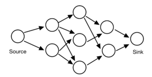
The given structure is a piping system. The water flows into the system from the source node, passing through the intermediate nodes, and flows out from the sink node. There is no limitation on the amount of water that can be used as the input for the source node. Therefore, the sink node can accept an unlimited amount of water coming into it. The arrows denote the valid channel that water can flow through, and each channel has a known flow capacity. What is the maximum flow that the system can take?
Several quantities should be defined to help formulate the frame of the solution:

For any intermediate node $ {\textstyle j } $ in the system, it receives water from adjacent node(s) $ i $, and sends water to the adjacent node(s) $ {\textstyle k } $. The node $ i $ and k are relative to the node $ {\textstyle j } $.
$ i $ = the node(s) that gives water to node $ {\textstyle j } $
$ {\textstyle j } $ = the intermediate node(s)
$ {\textstyle k } $ = the node(s) that receives the water coming out of node $ {\textstyle j } $
$ x_{ij} $ = amount of water leaving node $ i $ and entering node $ {\textstyle j } $ ($ i $ and $ {\textstyle j } $ are adjacent nodes)
$ x_{jk} $ = amount of water leaving node $ {\textstyle j } $ and entering node $ {\textstyle k } $ ($ i $ and $ {\textstyle k } $ are adjacent nodes)
For the source and sink node, they have net flow that is non-zero:
$ {\textstyle m } $ = source node
$ {\textstyle n } $ = sink node
$ x_{in} $ = amount of water leaving node $ i $ and entering sink node $ {\textstyle n } $ ($ i $ and $ {\textstyle n } $ are adjacent nodes)
$ x_{mk} $ = amount of water leaving source node $ {\textstyle m } $ and entering node $ {\textstyle k } $ ($ {\textstyle m } $ and $ {\textstyle k } $ are adjacent nodes)
Flow capacity definition is applied to all nodes (including intermediate nodes, the sink, and the source):
$ C_{ab} $ = transport capacity between any two nodes $ {\textstyle a } $ and $ {\textstyle b } $ ($ {\textstyle a } $$ \neq $$ {\textstyle b } $)
The main constraints for this problem are the transport capacity between each node and the material conservation:
(1): The amount of water flowing from any node $ {\textstyle a } $ to node $ {\textstyle b } $ should not exceed the flow capacity between node $ {\textstyle a } $ to node $ {\textstyle b } $ .
$ 0\leq x_{ab} \leq C_{ab} $
(2): The intermediate node $ {\textstyle j } $ does not hold any water, so the amount of water that flows into node $ {\textstyle j } $ has to exit the node with the exact same amount it entered with.
$ \sum_i^px_{ij}- \sum_k^r x_{jk} =0 \qquad \begin{cases} \forall i\in I=[1,p] \\ \forall j\in J=[1,q]\\ \forall k\in K=[1,r] \end{cases} $
Overall, the net flow out of the source node has to be the same as the net flow into the sink node. This net flow is the amount that should be maximized.
Using the definitions above:
min$ \quad z = \sum_k^r x_{uk} $ (or $ \sum_i^p x_{iv} $)
$ s.t. \quad\ \sum_i^px_{ij}- \sum_k^r x_{jk} =0 \qquad \begin{cases} \forall i\in I=[1,p] \\ \forall j\in J=[1,q]\\ \forall k\in K=[1,r] \end{cases} $
$ 0\leq x_{ab} \leq C_{ab} $
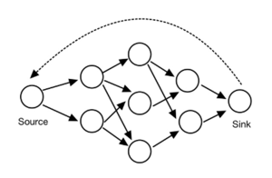
This expression can be further simplified by introducing an imaginary flow from the sink to the source.
By introducing this imaginary flow, the piping system is now closed. The mass conservation constraint now also holds for the source and sink node, so they can be treated as the intermediate nodes. The problem can be rewritten as the following:
min$ \quad z = x_{vu} $
$ s.t. \quad\ \sum_i^px_{ij}- \sum_k^r x_{jk} =0 \qquad \begin{cases} \forall i\in I=[1,p] \\ \forall j\in J=[1,q+2]\\ \forall k\in K=[1,r] \end{cases} $
$ 0\leq x_{ab} \leq C_{ab} $
The problem and the formulation are derived from an example in Chapter 8 of the book: Applied Mathematical Programming by Bradley, Hax and Magnanti. [3]
Algorithms
Ford–Fulkerson Algorithm
A broad range of network flow problems could be reduced to the max-flow problem. The most common way to approach the max-flow problem in polynomial time is the Ford-Fulkerson Algorithm (FFA). FFA is essentially a greedy algorithm and it iteratively finds the augmenting s-t path to increase the value of flow. The pathfinding terminates until there is no s-t path present. Ultimately, the max-flow pattern in the network graph will be returned. [8]
Typically, FFA is applied to flow networks with only one source node s and one sink node t. In addition, the capacity conditions and the conservation conditions, which are two properties defining the flow, must be satisfied.[9] The capacity conditions require that each edge carry a flow that is no more than its capacity, or $ 0\leq f(e)\leq c_{e},\forall e\in E $, where function f returns the flow on a certain edge. The conservation conditions require all nodes except the source and the sink to have a net flow of 0, or ,$ \sum_{e~into~v}f(v)= \sum_{e~out~of~v}f(v),\forall v\in V-{s,t} $.
FFA introduces the concept of residue graph based on the original graph $ G $ to allow backtracking, or pushing backward on edges that are already carrying flow.[9] The residue graph $ G_{f} $is defined as the following:
1. $ G_{f} $has exactly the same node set as $ G $.
2. For each edge $ e = (u,v) $with a nonnegative flow $ f( e) $ in $ G $, $ G_{f} $has the edge e with the capacity $ c(e)_{f} = c_{e} - f(e) $, and also $ G_f $ has the edge $ e' = (v,u) $ with the capacity $ c(e')_{f} = f(e) $.
Note that initially, the $ G_{f} $ is identical to $ G $ since there is no flow present in $ G $.
The steps of FFA are as below. [10] Essentially, the method repeatedly finds a path with positive flow in the residue graph, and updates the flow graph and residue graph until $ s $ and $ t $ become disjoint in the residue graph.
1. Set $ f(e) = 0, \forall e\in E $in $ G $, and create a copy as $ G_{f} $.
2. While there is still a $ s, t $ path $ p $ in $ G_{f} $:
a. Find $ c_{f}(p) = min(c_{f}(e):e\in p) $
b. For each edge $ e\in p $:
bi. $ f(e) = f(e) + c_{f}(p) $ if $ e\in E $ in $ G $, $ f(e) = f(e) - c_{f}(p) $ if $ e'\in E $ in $ G $
bii. $ c(e)= c(e) - c_{f}(p),c(e')= c(e') + c_{f}(p) $ in $ G_{f} $
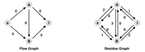
An example of running the FFA is as below. The flow graph $ G $ and residue graph$ G_{f} $ at the initial phase is depicted in Figure 8, where the number of each edge in the flow graph is the flow units on the edge, whereas it is the updated edge capacity in the residue graph.
In the residue graph, an $ s-t $ path can be found in the residue graph tracing the edge $ s\rightarrow A\rightarrow B\rightarrow t $ with the flow of two units. After augmenting the path on both graphs, the flow graph and the residue graph look like the Figure 9.
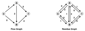
At this stage, there is still $ s,t $-path in the residue graph $ s\rightarrow B\rightarrow A\rightarrow t $ with a flow of one unit. After augmenting the path on both graphs, the flow graph and the residue graph look like the Figure 10.
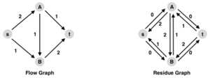
At this stage, there is no more $ s,t $-path in the residue graph, so FFA terminates and the maximum flow can be read from the flow graph as 3 units.
Numerical Example and Solution
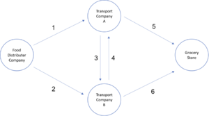
A Food Distributor Company is farming and collecting vegetables from farmers to later distribute to the grocery stores. The distributor has specific agreements with different third-party companies to mediate the delivery to the grocery stores. In a particular month, the company has 600 ton vegetables to deliver to the grocery store. They have agreements with two third-party transport companies A and B, which have different tariffs for delivering goods between themselves, the distributor, and the grocery store. They also have limits on transport capacity for each path. These delivery points are numbered as shown below, with path 1 being the transport from the Food Distributor Company to the transport company A. The limits and tariffs for each path can be found in the Table 2 below, and the possible transportation connections between the distributor company, the third-party transporters, and the grocery store are shown in the figure below. The distributor companies cannot hold any amount of food, and any incoming food should be delivered to an end point. The distributor company wants to minimize the overall transport cost of shipping 600 tons of vegetables to the grocery store by choosing the optimal path provided by the transport companies. How should the distributor company map out their path and the amount of vegetables carried on each path to minimize cost overall?
| 1 | 2 | 3 | 4 | 5 | 6 | |
| Product limit (ton) | 250 | 450 | 350 | 200 | 300 | 500 |
| Tariff ($/ton) | 10 | 12.5 | 5 | 7.5 | 10 | 20 |
This question is adapted from one of the exercise questions in chapter 8 of the book: Applied Mathematical Programming by Bradley, Hax and Magnanti [3].
Formulation of the Problem
The problem can be formulated as below where variables $ x_1, x_2, x_3,..., x_6 $ denote the tons of vegetables carried in paths 1 to 6. The objective function stated in the first line is to minimize the cost of the operation, which is the summation of the tons of vegetables carried on each path multiplied by the corresponding tariff: $ \sum_{i=1}^6 x_i t_i $.
$ \begin{array}{lcl} \min z = 10x_1 + 12.5x_2 + 5x_3 + 7.5x_4 + 10x_5 + 20x_6 \\ s.t. \qquad x_5 = x_1 - x_3 + x_4 \\ \ \ \ \quad \qquad x_6 = x_2 + x_3 - x_4 \\ \ \ \ \quad \qquad x_5 + x_6 = 600 \\ \ \ \ \quad \qquad x_1 + x_2 = 600 \\ \ \ \ \quad \qquad x_1 \leq 250 \\ \ \ \ \quad \qquad x_2 \leq 450 \\ \ \ \ \quad \qquad x_3 \leq 350 \\ \ \ \ \quad \qquad x_4 \leq 200 \\ \ \ \ \quad \qquad x_5 \leq 300 \\ \ \ \ \quad \qquad x_6 \leq 500 \\ \ \ \ \quad \qquad x_1, x_2, x_3, x_4, x_5, x_6 \geq 0\\\end{array} $
The second step is to write down the constraints. The first constraint ensures that the net amount present in the Transport Company A, which is the deliveries received from path 1 and path 2 minus the transport to Transport Company B should be delivered to the grocery store with path 5. The second constraint ensures this for the Transport Company B. The third and fourth constraints are ensuring that the total amount of vegetables shipping from the Food Distributor Company and the total amount of vegetables delivered to the grocery store are both 600 tons. The constraints 5 to 10 depict the upper limits of the amount of vegetables that can be carried on paths 1 to 6. The final constraint depicts that all variables are non-negative.
Solution of the Problem
This problem can be solved using Simplex Algorithm[11] or with the CPLEX Linear Programming solver in GAMS optimization platform. The steps of the solution using the GAMS platform is as follows:
The first step is to list the variables, which are the tons of vegetables that will be transported in routes 1 to 6. The paths can be denoted as$ x_1, x_2, x_3,..., x_6 $ . The objective function is the overall cost: z.
variables x1,x2,x3,x4,x5,x6,z;
The second step is to list the equations which are the constraints and the objective function. The objective function is a summation of the amount of vegetables carried in path i, multiplied with the tariff of path i for all i: $ \sum_{i=1}^6 x_i t_i $. The GAMS code for the objective function is written below:
obj.. z=e= 10*x1+12.5*x2+5*x3+7.5*x4+10*x5+20*x6;
Overall, there are 10 constraints in this problem. The constraints 1, and 2 are equations for the paths 5 and 6. The amount carried in path 5 can be found by summing the amount of vegetables incoming to Transport Company A from path 1 and path 4, minus the amount of vegetables leaving Transport Company A with path 3. This can be attributed to the restriction that barrs the companies from keeping any vegetables and requires them to eventually deliver all the incoming produce. The equality 1 ensures that this constraint holds for path 5 and equation 2 ensures it for path 6. A sample of these constraints is written below for path 5:
c1.. x5 =e=x1-x3+x4;
Constraint 3 ensures that the sum of vegetables carried in path 1 and path 2 add to the total of 600 tons of vegetables that leave the Food Distributor Company. Likewise, the constraint 4 ensures that the sum amount of food transported in paths 5 and 6 adds up to 600 tons of vegetables that have to be delivered to the grocery store. A sample of these constraints is written below for the total delivery to the grocery store:
c3.. x5+x6=e=600;
Constraints 5 to 10 should ensure that the amount of food transported in each path should not exceed the maximum capacity depicted in the table. A sample of these constraints is written below for the capacity of path 1:
c5.. x1=l=250;
After listing the variables, objective function and the constraints, the final step is to call the CPLEX solver and set the type of the optimization problem as lp (linear programming). In this case the problem will be solved with a Linear Programming algorithm to minimize the objective (cost) function.
The GAMS code yields the results below:
x1 = 250, x2 = 350, x3 = 0, x4 = 50, x5 = 300, x6 = 300, z =16250.
Real Life Applications
Network problems have many applications in all kinds of areas such as transportation, city design, resource management and financial planning.[6]
There are several special cases of network problems, such as the shortest path problem, minimum cost flow problem, assignment problem and transportation problem.[6] Three application cases will be introduced here.
The Minimum Cost Flow Problem
Minimum cost flow problems are pervasive in real life, such as deciding how to allocate temporal quay crane in container terminals, and how to make optimal train schedules on the same railroad line.[12]
R. Dewil and his group use MCNFP to assist traffic enforcement.[13] Police patrol “hot spots”, which are areas where crashes occur frequently on highways. R. Dewil studies a method intended to estimate the optimal route of hot spots. He describes the time it takes to move the detector to a certain position as the cost, and the number of patrol cars from one node to next as the flow, in order to minimize the total cost.[13]
The Assignment Problem
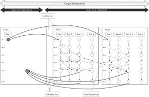
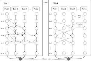
Dung-Ying Lin studies an assignment problem in which he aims to assign freights to ships and arrange transportation paths along the Northern Sea Route in a manner which yields maximum profit.[14] Within this network composed of a ship subnetwork and a cargo subnetwork( shown as Figure 12 and Figure 13), each node corresponds to a port at a specific time and each arc represents the movement of a ship or a cargo. Other types of assignment problems are faculty scheduling, freight assignment, and so on.
The Shortest Path Problem
Shortest path problems are also present in many fields, such as transportation, 5G wireless communication, and implantation of the global dynamic routing scheme.[15][16][17]
Qiang Tu and his group studies the constrained reliable shortest path (CRSP) problem for electric vehicles in the urban transportation network. [15] He describes the reliable travel time of path as the objective item, which is made up of planning travel time of path and the reliability item. The group studies the Chicago sketch network consisting of 933 nodes and 2950 links and the Sioux Falls network consisting of 24 nodes and 76 links. The results show that the travelers’ risk attitudes and properties of electric vehicles in the transportation network can have a great influence on the path choice.[15] The study can contribute to the invention of the city navigation system.
Conclusion
Since its inception, the network flow problem has provided humanity with a straightforward and scalable approach for several large-scale challenges and problems. The Simplex algorithm and other computational optimization platforms have made addressing these problems routine, and have greatly expedited efforts for groups concerned with supply-chain and other distribution processes. The formulation of this problem has had several derivations from its original format, but its overall methodology and approach have remained prevalent in several of society’s industrial and commercial processes, even over half a century later. Classical models such as the assignment, transportation, maximal flow, and shortest path problem configurations have found their way into diverse settings, ranging from streamlining oil distribution networks along the gulf coast to arranging optimal scheduling assignments for college students amidst a global pandemic. All in all, the network flow problem and its monumental impact, have made it a fundamental tool for any group that deals with combinatorial data sets. And with the surge in adoption of data-driven models and applications within virtually all industries, the use of the network flow problem approach will only continue to drive innovation and meet consumer demands for the foreseeable future.
References
1. Karp, R. M. (2008). George Dantzig’s impact on the theory of computation. Discrete Optimization, 5(2), 174-185.
2. Goldberg, A. V. Tardos, Eva, Tarjan, Robert E. (1989). Network Flow Algorithms, Algorithms and Combinatorics. 9. 101-164.
3. Bradley, S. P. Hax, A. C., & Magnanti, T. L. (1977). Network Models. Applied mathematical programming (p. 259). Reading, MA: Addison-Wesley.
4. Chinneck, J. W. (2006). Practical optimization: a gentle introduction. Systems and Computer Engineering. Carleton University, Ottawa. 11.
5. Roy, B. V. Mason, K.(2005). Formulation and Analysis of Linear Programs, Chapter 5 Network Flows.
6. Vanderbei, R. J. (2020). Linear programming: foundations and extensions (Vol. 285). Springer Nature.
7. Sobel, J. (2014). Linear Programming Notes VIII: The Transportation Problem.
8. Cormen, Thomas H.; Leiserson, Charles E.; Rivest, Ronald L.; Stein, Clifford (2001). "Section 26.2: The Ford–Fulkerson method". Introduction to Algorithms (Second ed.). MIT Press and McGraw–Hill.
9. Jon Kleinberg; Éva Tardos (2006). "Chapter 7: Network Flow". Algorithm Design. Pearson Education.
10. Ford–Fulkerson algorithm. Retrieved December 05, 2020.
11. Hu, G. (2020, November 19). Simplex algorithm. Retrieved November 22, 2020.
12. Altınel, İ. K., Aras, N., Şuvak, Z., & Taşkın, Z. C. (2019). Minimum cost noncrossing flow problem on layered networks. Discrete Applied Mathematics, 261, 2-21.
13. Dewil, R., Vansteenwegen, P., Cattrysse, D., & Van Oudheusden, D. (2015). A minimum cost network flow model for the maximum covering and patrol routing problem. European Journal of Operational Research, 247(1), 27-36.
14. Lin, D. Y., & Chang, Y. T. (2018). Ship routing and freight assignment problem for liner shipping: Application to the Northern Sea Route planning problem. Transportation Research Part E: Logistics and Transportation Review, 110, 47-70.
15. Tu, Q., Cheng, L., Yuan, T., Cheng, Y., & Li, M. (2020). The Constrained Reliable Shortest Path Problem for Electric Vehicles in the Urban Transportation Network. Journal of Cleaner Production, 121130.
16. Guo, Y., Li, S., Jiang, W., Zhang, B., & Ma, Y. (2017). Learning automata-based algorithms for solving the stochastic shortest path routing problems in 5G wireless communication. Physical Communication, 25, 376-385.
17. Haddou, N. B., Ez-Zahraouy, H., & Rachadi, A. (2016). Implantation of the global dynamic routing scheme in scale-free networks under the shortest path strategy. Physics Letters A, 380(33), 2513-2517.