Wing shape optimization: Difference between revisions
| (8 intermediate revisions by 2 users not shown) | |||
| Line 23: | Line 23: | ||
One problem is presented at two different levels of complexity. The objective is to maximum the coefficient of lift of a 2-D airfoil starting from the NACA 0012 profile (a common profile developed by the National Advisory Committee for Aeronautics). The actual problem being solved is developed in the open-source CFD package OpenFOAM (Open Source Field Operation and Manipulation) with results presented. The simplified version is presented here in depth to illustrate the process of wing shape optimization.[[File:Naca0012-1.jpg|thumb|'''Figure 2.''' Initial parameterized airfoil]]The problem formulation begins with the initial airfoil design being parameterized with points defined by x and y coordinates – these coordinates are contained in the <math>\boldsymbol{\beta} </math> vector. In this case, the x coordinates are fixed, so <math>\boldsymbol{\beta} </math> only contains y values. The objective of this problem is to maximize the lift produced by the airfoil. | One problem is presented at two different levels of complexity. The objective is to maximum the coefficient of lift of a 2-D airfoil starting from the NACA 0012 profile (a common profile developed by the National Advisory Committee for Aeronautics). The actual problem being solved is developed in the open-source CFD package OpenFOAM (Open Source Field Operation and Manipulation) with results presented. The simplified version is presented here in depth to illustrate the process of wing shape optimization.[[File:Naca0012-1.jpg|thumb|upright=1.2|'''Figure 2.''' Initial parameterized airfoil]]The problem formulation begins with the initial airfoil design being parameterized with points defined by x and y coordinates – these coordinates are contained in the <math>\boldsymbol{\beta} </math> vector. In this case, the x coordinates are fixed, so <math>\boldsymbol{\beta} </math> only contains y values. The objective of this problem is to maximize the lift produced by the airfoil. | ||
<math>J = J(\boldsymbol{v}, p, \boldsymbol{\beta}) = - \oint p \hat{n} \sin(\theta) dS </math> | <math>J = J(\boldsymbol{v}, p, \boldsymbol{\beta}) = - \oint p \hat{n} \sin(\theta) dS </math> | ||
Where '''<math>\boldsymbol{v} </math>''' is the vector of velocity magnitudes in the x and y directions, <math>p </math> is pressure, and <math>\boldsymbol{\beta} </math> is the vector containing the y coordinates that parameterize the airfoil. To determine the lift produced by the airfoil, a computational mesh must be created surrounding the airfoil. In each of the cells of the mesh, the governing equations of fluid mechanics, conservation of mass (Navier-Stokes) and conservation of mass (continuity), must be solved. This means that each variable in the objective equations (and the constraints), '''<math>\boldsymbol{v} </math>''', <math>p </math>, and <math>\boldsymbol{\beta} </math>, are vectors of the length equal to the number of cells in the computational domain (often in the range from 1e3 to 1e7). This is done in a CFD package, specifically OpenFOAM in this case, and is not the focus of this numerical example. Conservation of momentum and conservation of mass form the constraints. Additionally, in this case, a maximum value for coefficient of drag is chosen. (Note that the simulation has boundary conditions that must also be satisfied, i.e., specified inlet velocity, but these are typically not listed as optimization constraints.) | Where '''<math>\boldsymbol{v} </math>''' is the vector of velocity magnitudes in the x and y directions, <math>p </math> is pressure, and <math>\boldsymbol{\beta} </math> is the vector containing the y coordinates that parameterize the airfoil. To determine the lift produced by the airfoil, a computational mesh must be created surrounding the airfoil. In each of the cells of the mesh, the governing equations of fluid mechanics, conservation of mass (Navier-Stokes) and conservation of mass (continuity), must be solved. This means that each variable in the objective equations (and the constraints), '''<math>\boldsymbol{v} </math>''', <math>p </math>, and <math>\boldsymbol{\beta} </math>, are vectors of the length equal to the number of cells in the computational domain (about 3e6 cells in this case; often in the range from 1e3 to 1e7). This is done in a CFD package, specifically OpenFOAM in this case, and is not the focus of this numerical example. Conservation of momentum and conservation of mass form the constraints. Additionally, in this case, a maximum value for coefficient of drag is chosen. (Note that the simulation has boundary conditions that must also be satisfied, i.e., specified inlet velocity, but these are typically not listed as optimization constraints.) | ||
<math>\boldsymbol{R} (\boldsymbol{v} , p , \boldsymbol{\beta} ) = 0 | |||
</math> | |||
<math>(R_1, R_2, R_3)^T = ( \boldsymbol{v} \cdot \nabla ) \boldsymbol{v} + \nabla p - \nu \nabla^2 (\boldsymbol{v})</math> | |||
<math>R_4 = - \nabla \boldsymbol{u}</math><ref name=":1" /> | |||
Besides solving the physics of the fluid surrounding the airfoil, the airfoil design producing the most lift must also be solved using an optimization method. In this case, the steepest descent method is used because that is the method used by the solver adjointOptimisationFoam in OpenFOAM and the initial NACA 0012 airfoil is assumed to be close to the optimal design. | Besides solving the physics of the fluid surrounding the airfoil, the airfoil design producing the most lift must also be solved using an optimization method. In this case, the steepest descent method is used because that is the method used by the solver adjointOptimisationFoam in OpenFOAM and the initial NACA 0012 airfoil is assumed to be close to the optimal design. | ||
<math>\boldsymbol{\beta}_{N+1} = \boldsymbol{\beta}_{N} + \alpha \centerdot \delta L </math> | <math>\boldsymbol{\beta}_{N+1} = \boldsymbol{\beta}_{N} + \alpha \centerdot \delta L </math><ref name=":1" /> | ||
Where <math>\boldsymbol{\beta}_{N} </math> are the current coordinates, <math>\boldsymbol{\beta}_{N+1} </math> are the next coordinates, and <math>\alpha </math> is the time step. The <math>\delta L </math> term is the variation in the Lagrange function <math>L </math> which combines the objective and constraints multiped by Lagrange multipliers called adjoint variables. This is not discussed in detail here, but essentially, by creating the Lagrange function, it can be manipulated so that the objective only depends on the airfoil shape, the entire flow domain does not need to be solved every optimization iteration. | Where <math>\boldsymbol{\beta}_{N} </math> are the current coordinates, <math>\boldsymbol{\beta}_{N+1} </math> are the next coordinates, and <math>\alpha </math> is the time step. The <math>\delta L </math> term is the variation in the Lagrange function <math>L </math> which combines the objective and constraints multiped by Lagrange multipliers called adjoint variables. This is not discussed in detail here, but essentially, by creating the Lagrange function, it can be manipulated so that the objective only depends on the airfoil shape, the entire flow domain does not need to be solved every optimization iteration. | ||
Although changes in the position of airfoil coordinates are not visible after just one iteration, after multiple iterations, you can see the y coordinates of the airfoil start to “move”. | Although changes in the position of airfoil coordinates are not visible after just one iteration, after multiple iterations, you can see the y coordinates of the airfoil start to “move”. | ||
[[File:Naca0012-2.jpg|thumb|center|'''Figure 3.''' Airfoil parameterization after multiple iterations]] | [[File:Naca0012-2.jpg|thumb|center|upright=1.2|'''Figure 3.''' Airfoil parameterization after multiple iterations]] | ||
After nearly fifteen thousand optimization iterations in OpenFOAM, the solution converged. | After nearly fifteen thousand optimization iterations in OpenFOAM, the solution converged. | ||
[[File:PressureContours-5.png|thumb|right|upright=1.45|'''Figure 5. Pressure contours of optimized airfoil''']] | [[File:PressureContours-5.png|thumb|right|upright=1.45|'''Figure 5. Pressure contours of optimized airfoil''']] | ||
| Line 50: | Line 54: | ||
From the contour plots, the pressure is significantly greater of the bottom of the airfoil in Figure 5 than Figure 4. This pressure difference resulted in an increase of approximately 2% in the coefficient of lift. | From the contour plots, the pressure is significantly greater of the bottom of the airfoil in Figure 5 than Figure 4. This pressure difference resulted in an increase of approximately 2% in the coefficient of lift. | ||
[[File:Airfoil-1.png|thumb| | [[File:Airfoil-1.png|thumb|center|upright=1.49|'''Figure 6.''' Original airfoil]] | ||
[[File:Airfoil-5.png|thumb| | [[File:Airfoil-5.png|thumb|center|upright=1.49|'''Figure 7.''' Optimized airfoil]] | ||
== Applications == | == Applications == | ||
| Line 74: | Line 78: | ||
==Conclusion== | ==Conclusion== | ||
With the various uses of wing-shape optimization, it is abundantly clear that this optimization method is robust enough to withstand most problems that carry real world constraints/parameters. The shape of a blade or a wing is subjected to a wide variety of dimensional and performance constraints, magnifying the need to correctly set up one’s optimization problem. These constraints then directly affect the outcome of the objective, such as optimizing aerodynamic performance through drag and lift coefficient constraining. By reducing the drag coefficient of the solution, one also reduces the amount of generated lift, expectedly lowering an aircraft in altitude<ref>ZADEH, Parviz MOHAMMAD, and Mohsen Sayadi. "An efficient aerodynamic shape optimization of blended wing body UAV using multi-fidelity models." Chinese Journal of Aeronautics 31.6 (2018): 1165-1180.</ref>. Another constraint that factors into this optimization is the wing length, which can be constrained due to a physical or monetary/material constraint. As seen, certain regulatory factors have to be followed for the solution to be feasible, but there are other driving factors that are out of engineering control. | With the various uses of wing-shape optimization, it is abundantly clear that this optimization method is robust enough to withstand most problems that carry real world constraints/parameters. The shape of a blade or a wing is subjected to a wide variety of dimensional and performance constraints, magnifying the need to correctly set up one’s optimization problem. These constraints then directly affect the outcome of the objective, such as optimizing aerodynamic performance through drag and lift coefficient constraining. By reducing the drag coefficient of the solution, one also reduces the amount of generated lift, expectedly lowering an aircraft in altitude<ref>ZADEH, Parviz MOHAMMAD, and Mohsen Sayadi. "An efficient aerodynamic shape optimization of blended wing body UAV using multi-fidelity models." Chinese Journal of Aeronautics 31.6 (2018): 1165-1180.</ref>. Another constraint that factors into this optimization is the wing length, which can be constrained due to a physical or monetary/material constraint. Using the example provided in the Applications Section regarding airwing optimization, across-sectional areas of wings also greatly affect the constraints needed to be satisfied. As seen, certain regulatory factors have to be followed for the solution to be feasible, but there are other driving factors that are out of engineering control. | ||
<math display="inline">\begin{array}{lcl} C_D & = & {C_L^2 \over \pi*AR*e} \\ C_D & = & Drag \ Coefficient \\ C_L & = & Lift \ Coefficient \\ AR & = & Aspect \ Ratio \\ e & = & Efficiency \ Factor \end{array}</math><ref>“Induced Drag Coefficient.” NASA, NASA, <nowiki>https://www.grc.nasa.gov/www/k-12/airplane/induced.html</nowiki>.</ref> | <math display="inline">\begin{array}{lcl} C_D & = & {C_L^2 \over \pi*AR*e} \\ C_D & = & Drag \ Coefficient \\ C_L & = & Lift \ Coefficient \\ AR & = & Aspect \ Ratio \\ e & = & Efficiency \ Factor \end{array}</math><ref>“Induced Drag Coefficient.” NASA, NASA, <nowiki>https://www.grc.nasa.gov/www/k-12/airplane/induced.html</nowiki>.</ref> | ||
Latest revision as of 00:59, 16 December 2021
Authors: Santiago Correa, Jeet Dhoriyani, Joshua Krsek, Aayush Singh, Jeremy Wang (SYSEN/CHEME 6800 Fall 2021)
Introduction
The aerodynamic performance of a given body is optimized using an aerodynamic shape optimization method. This process can be thought of as minimizing the cost of total fuel consumption and maximizing the total lift of an aircraft by a method known as wing shape optimization. The aerodynamic performance is evaluated using methods like computational fluid dynamics[1]and the optimization can be done using a number of algorithms like the adjoint method, direct sensitivity analysis and finite difference. The wing shape problem is an application under the aerodynamic shape optimization method. An adjoint method also known as gradient-based method is often used for shape optimization which is capable of computing objective function sensitivities based on the design parameters and variables of the shape under investigation. The discrete formulation is used for the purpose of explanation in this wiki.The discrete-adjoint Method used for the aerodynamic optimization aims at computing the gradient of the objective function with respect to the design variable.
Theory, methodology, and/or algorithmic discussions
To perform wing shape optimization, two tools must be utilized simultaneously – a differential equation solver used to solve the parameters of the fluid flow (often a computational fluid dynamics (CFD) package) and an optimization method that adjusts the wing shape parameters to achieve an optimum of a specific quantity.[2]
Shape parameterization
There are numerous commercial and open-source CFD programs capable of resolving air flow around an airplane wing. The new methods introduced when discussing wing shape optimization, or shape optimization in general, are the optimization methods that modify the shape to achieve a desired minimum or maximum quantity subject to specified constraints. In order to modify the shape of the airfoil or overall wing, the original shape must be defined mathematically in a way that allows it to be update within an optimization loop. One method is to discretize the airfoil shape in to points defined by x and y coordinates, which become the design parameters updated each optimization iteration. This method allows for nearly any shape to be formed because the points can move in any direction. However, this can sometimes result in sharp corner in the airfoil which are difficult to resolve by the flow solver. Furthermore, storing a high-resolution shape, meaning a large number of points, is computationally expensive.[3] Another shape parametrization method is to define the airfoil using two polynomials, one for the top surface, one for the bottom. For this method, the degree n of the polynomial is determined by defining the initial airfoil shape. The design parameters are the weights in front of each $ x^n $ term.[3]
$ y(x) = w_0 \sqrt{x} + w_1 x + w_2 x^2 + w_3 x^3 + w_4 x^4 $
Mesh moving
When the shape of the airfoil changes with each optimization iteration, the mesh defining the flow domain around the airfoil must adjust according. Two methods are typically used to update the mesh. For large changes in shape, the entire flow domain can be re-meshed for the new shape present using a variety of mesh techniques. This is quite computationally expensive, especially for large or high-resolution domains. The other method is to simply move cells to account for the change in shape. To prevent potential overlapping of cells from this movement, splines are often defined from the surface of the shape to the boundary of the domain which the cells move.[4]
Optimization
Multiple optimization techniques are used update the design parameters and achieve the minimum or maximum specified quantity, such as the adjoint method, direct sensitivity analysis and finite difference. The adjoint method is the most common method due to its computational independence from the number of design variables. The adjoint method initially solves for the flow parameters in the flow domain. However, after these parameters are initially solved, they do not need to be recomputed because the adjoint gradient which updates the design parameters is independent of the flow parameters. This is unique to the adjoint method is why it is commonly used instead of the computationally intensive finite difference method.[4]
Numerical example
As previously mentioned, wing shape optimization is a complex procedure which can be applied to full 3-D wings to achieve optimal results for a plethora of objectives. The example presented below of optimizing a 2-D airfoil to achieve maximum lift is a simple case in the scope of wing shape optimization; however, it is quite extensive in comparison to other optimization problems.
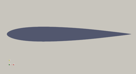
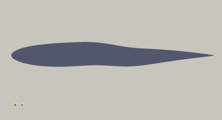
One problem is presented at two different levels of complexity. The objective is to maximum the coefficient of lift of a 2-D airfoil starting from the NACA 0012 profile (a common profile developed by the National Advisory Committee for Aeronautics). The actual problem being solved is developed in the open-source CFD package OpenFOAM (Open Source Field Operation and Manipulation) with results presented. The simplified version is presented here in depth to illustrate the process of wing shape optimization.

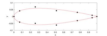
The problem formulation begins with the initial airfoil design being parameterized with points defined by x and y coordinates – these coordinates are contained in the $ \boldsymbol{\beta} $ vector. In this case, the x coordinates are fixed, so $ \boldsymbol{\beta} $ only contains y values. The objective of this problem is to maximize the lift produced by the airfoil.
$ J = J(\boldsymbol{v}, p, \boldsymbol{\beta}) = - \oint p \hat{n} \sin(\theta) dS $
Where $ \boldsymbol{v} $ is the vector of velocity magnitudes in the x and y directions, $ p $ is pressure, and $ \boldsymbol{\beta} $ is the vector containing the y coordinates that parameterize the airfoil. To determine the lift produced by the airfoil, a computational mesh must be created surrounding the airfoil. In each of the cells of the mesh, the governing equations of fluid mechanics, conservation of mass (Navier-Stokes) and conservation of mass (continuity), must be solved. This means that each variable in the objective equations (and the constraints), $ \boldsymbol{v} $, $ p $, and $ \boldsymbol{\beta} $, are vectors of the length equal to the number of cells in the computational domain (about 3e6 cells in this case; often in the range from 1e3 to 1e7). This is done in a CFD package, specifically OpenFOAM in this case, and is not the focus of this numerical example. Conservation of momentum and conservation of mass form the constraints. Additionally, in this case, a maximum value for coefficient of drag is chosen. (Note that the simulation has boundary conditions that must also be satisfied, i.e., specified inlet velocity, but these are typically not listed as optimization constraints.)
$ \boldsymbol{R} (\boldsymbol{v} , p , \boldsymbol{\beta} ) = 0 $
$ (R_1, R_2, R_3)^T = ( \boldsymbol{v} \cdot \nabla ) \boldsymbol{v} + \nabla p - \nu \nabla^2 (\boldsymbol{v}) $
$ R_4 = - \nabla \boldsymbol{u} $[4]
Besides solving the physics of the fluid surrounding the airfoil, the airfoil design producing the most lift must also be solved using an optimization method. In this case, the steepest descent method is used because that is the method used by the solver adjointOptimisationFoam in OpenFOAM and the initial NACA 0012 airfoil is assumed to be close to the optimal design.
$ \boldsymbol{\beta}_{N+1} = \boldsymbol{\beta}_{N} + \alpha \centerdot \delta L $[4]
Where $ \boldsymbol{\beta}_{N} $ are the current coordinates, $ \boldsymbol{\beta}_{N+1} $ are the next coordinates, and $ \alpha $ is the time step. The $ \delta L $ term is the variation in the Lagrange function $ L $ which combines the objective and constraints multiped by Lagrange multipliers called adjoint variables. This is not discussed in detail here, but essentially, by creating the Lagrange function, it can be manipulated so that the objective only depends on the airfoil shape, the entire flow domain does not need to be solved every optimization iteration.
Although changes in the position of airfoil coordinates are not visible after just one iteration, after multiple iterations, you can see the y coordinates of the airfoil start to “move”.
After nearly fifteen thousand optimization iterations in OpenFOAM, the solution converged.
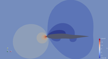
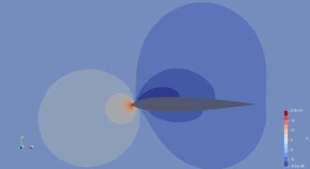
From the contour plots, the pressure is significantly greater of the bottom of the airfoil in Figure 5 than Figure 4. This pressure difference resulted in an increase of approximately 2% in the coefficient of lift.
Applications
Aircraft wing shape optimization for wing mounted models
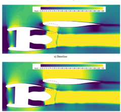
Wing-mounted configuration is very common in modern civil aircraft because of many advantages. For example, the wings structure is unloaded by the engine’s weight in flights, and the passenger cabin gets a low noise level. Furthermore, this configuration also contributes to the easy maintenance and replacement of the power systems. For given wing shape the gradient-based optimization system is commonly used. The CFD mesh and FFD block is generated, and they are passed to the optimizer to define the aerodynamic optimization problem, such as drag minimization with respect to lift. The discrete-Adjoin Method is chosen to fulfill the complex aerodynamic optimization. problems. After the optimization problem is defined, the design variables vector is determined by the optimizer and passed to the shape parameterization module to produce a new surface mesh. [6]
Blended wing body optimization for Unmanned Aerial Vehicle (UAV)
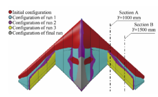
In recent years, in order to reduce fuel consumption and improve performance, the optimization of UAV shapes has been the main focus of the competitive aerospace market. The development of Blended Wing Body (BWB) design is such an effort. In addition to the elimination of the tail for this particular kind of UAV and the significant reduction in equivalent weight, drag force, and radar cross-section, the available space for installing equipment inside the wing and the effective range have also been increased. [8]
Drone propeller topology optimization
The propeller is a type of fan that converts mechanical energy into thrust power by accelerating the propulsive fluid. A drone propeller optimized the geometry to achieve greater efficiency and therefore longer life of multirotor adopts these propellers. Optimized propeller designs also help in saving the battery life of electric drones.[9]
Wind turbine blade optimization
An aerodynamically efficient blade is the prime necessity to extract maximum power from a wind turbine. With the increasing size of the wind turbine blade, the blades are now basically made of composite materials. In the research on the structure of wind turbine blades, the study of structural testing and simulation of the wind turbine blade. The overall goal is to reduce the cost price of the produced power, and as long a size increase results in lowering the cost price, the trend will continue. However, another way of capturing more wind energy is to improve the aerodynamic efficiency of the energy conversion, such as maximizing the power coefficient and the energy yield of wind turbines. [10]
Conclusion
With the various uses of wing-shape optimization, it is abundantly clear that this optimization method is robust enough to withstand most problems that carry real world constraints/parameters. The shape of a blade or a wing is subjected to a wide variety of dimensional and performance constraints, magnifying the need to correctly set up one’s optimization problem. These constraints then directly affect the outcome of the objective, such as optimizing aerodynamic performance through drag and lift coefficient constraining. By reducing the drag coefficient of the solution, one also reduces the amount of generated lift, expectedly lowering an aircraft in altitude[11]. Another constraint that factors into this optimization is the wing length, which can be constrained due to a physical or monetary/material constraint. Using the example provided in the Applications Section regarding airwing optimization, across-sectional areas of wings also greatly affect the constraints needed to be satisfied. As seen, certain regulatory factors have to be followed for the solution to be feasible, but there are other driving factors that are out of engineering control.
$ {\textstyle \begin{array}{lcl} C_D & = & {C_L^2 \over \pi*AR*e} \\ C_D & = & Drag \ Coefficient \\ C_L & = & Lift \ Coefficient \\ AR & = & Aspect \ Ratio \\ e & = & Efficiency \ Factor \end{array}} $[12]
When constraining a wing turbine blade, engineers need to also factor in the length of the blade along with the strength of the building material to ensure the blade does not snap during use at any wing speed[13]. The designed blade would need to stay intact during periods of no wind to periods of strong wind due to inclement weather. This is a factor that needs to be considered when constructing the optimization algorithm, which highlights the importance of the correct problem setup. If an optimization algorithm is unable to solve the basic problem ensuring component integrity, then it is presumed the solution will fare poorly in a more complicated performance analysis/situation.
Having the correct optimization algorithm is critical to the success of the solution. If a certain constraint is missed or forgotten, the entire solution is at risk of failure due to this simple mistake. This is one of the small number drawbacks to wing-shape optimization, the real world implication of the solution and ensuring its high performance during prototyping and testing. Nevertheless, wing shape optimization through Adjoint Method, Direct Sensitivity Analysis or Finite Differences is a versatile solution methodology as all factors can be coded as constraints and the solution will fulfill the objective of the project. The solution also satisfies all real world factors that have been coded to ensure the most optimized feasible solution.
References
- ↑ Blazek, J. Computational Fluid Dynamics: Principles and Applications (Third Edition). Butterworth-Heinemann.
- ↑ Ping He, Charles A. Mader, Joaquim R. R. A. Martins, and Kevin J. Maki. An aerodynamic design optimization framework using a discrete adjoint approach with OpenFOAM. Computers & Fluids, 168 (2018) 285–303. doi: 10.1016/j.compfluid.2018.04.012
- ↑ 3.0 3.1 Silisteanu, Paul & Botez, Ruxandra. (2012). Two-dimensional airfoil shape optimization for airfoils at low speeds. AIAA Modeling and Simulation Technologies Conference 2012. 10.2514/6.2012-4790.
- ↑ 4.0 4.1 4.2 4.3 4.4 Schramm, Matthias & Stoevesandt, Bernhard & Peinke, Joachim. (2018). Optimization of Airfoils Using the Adjoint Approach and the Influence of Adjoint Turbulent Viscosity. Computation. 6. 5. 10.3390/computation6010005.
- ↑ Lei, Ruiwu, Junqiang Bai, and Danyang Xu. "Aerodynamic optimization of civil aircraft with wing-mounted engine jet based on adjoint method." Aerospace Science and Technology 93 (2019): 105285.
- ↑ Lei, Ruiwu, Junqiang Bai, and Danyang Xu. "Aerodynamic optimization of civil aircraft with wing-mounted engine jet based on adjoint method." Aerospace Science and Technology 93 (2019): 105285.
- ↑ Lei, Ruiwu, Junqiang Bai, and Danyang Xu. "Aerodynamic optimization of civil aircraft with wing-mounted engine jet based on adjoint method." Aerospace Science and Technology 93 (2019): 105285.
- ↑ ZADEH, Parviz MOHAMMAD, and Mohsen Sayadi. "An efficient aerodynamic shape optimization of blended wing body UAV using multi-fidelity models." Chinese Journal of Aeronautics 31.6 (2018): 1165-1180.
- ↑ LAROCCA, Francesco, et al. "Topological optimization of a drone propeller using commercial CFD code."
- ↑ Song, Fangfang, Yihua Ni, and Zhiqiang Tan. "Optimization design, modeling and dynamic analysis for composite wind turbine blade." Procedia Engineering 16 (2011): 369-375.
- ↑ ZADEH, Parviz MOHAMMAD, and Mohsen Sayadi. "An efficient aerodynamic shape optimization of blended wing body UAV using multi-fidelity models." Chinese Journal of Aeronautics 31.6 (2018): 1165-1180.
- ↑ “Induced Drag Coefficient.” NASA, NASA, https://www.grc.nasa.gov/www/k-12/airplane/induced.html.
- ↑ Song, Fangfang, Yihua Ni, and Zhiqiang Tan. "Optimization design, modeling and dynamic analysis for composite wind turbine blade." Procedia Engineering 16 (2011): 369-375.