Heuristic algorithms: Difference between revisions
No edit summary |
|||
| (12 intermediate revisions by the same user not shown) | |||
| Line 23: | Line 23: | ||
* '''Metaheuristics''', such as simulated annealing or genetic algorithms, tackle the TSP by employing high-level strategies to explore the solution space more broadly and escape local optima. These methods balance global search space exploration with local exploitation of promising regions, allowing for a more thorough search for better solutions. They iteratively improve the solution while occasionally considering less favorable configurations to avoid being confined to suboptimal areas. By guiding the search process intelligently, metaheuristics adapt dynamically and effectively solve the TSP, often producing near-optimal solutions even for large-scale or complex problem instances. | * '''Metaheuristics''', such as simulated annealing or genetic algorithms, tackle the TSP by employing high-level strategies to explore the solution space more broadly and escape local optima. These methods balance global search space exploration with local exploitation of promising regions, allowing for a more thorough search for better solutions. They iteratively improve the solution while occasionally considering less favorable configurations to avoid being confined to suboptimal areas. By guiding the search process intelligently, metaheuristics adapt dynamically and effectively solve the TSP, often producing near-optimal solutions even for large-scale or complex problem instances. | ||
==Popular | == Popular Optimization Heuristics Algorithms == | ||
=== Heuristic | === '''Heuristic Algorithms''' === | ||
==== '''Constructive Algorithm (Greedy)''' ==== | |||
=== '''Constructive Algorithm (Greedy)''' === | |||
'''Constructive heuristics''' are algorithmic strategies that build solutions incrementally, starting from an empty set and adding elements sequentially until a complete and feasible solution is formed (greedy algorithms). This approach is particularly advantageous due to its simplicity in design, analysis, implementation and limited computational complexity. However, the quality of solutions produced by constructive heuristics heavily depends on the criteria used for adding elements, and they may only sometimes yield optimal results.<ref>Aringhieri, R., Cordone, R., Guastalla, A., Grosso, A. (2023). Constructive and Destructive Methods in Heuristic Search. In: Martí, R., Martínez-Gavara, A. (eds) Discrete Diversity and Dispersion Maximization. Springer Optimization and Its Applications, vol 204. Springer, Cham. https://doi.org/10.1007/978-3-031-38310-6_4.</ref> | '''Constructive heuristics''' are algorithmic strategies that build solutions incrementally, starting from an empty set and adding elements sequentially until a complete and feasible solution is formed (greedy algorithms). This approach is particularly advantageous due to its simplicity in design, analysis, implementation and limited computational complexity. However, the quality of solutions produced by constructive heuristics heavily depends on the criteria used for adding elements, and they may only sometimes yield optimal results.<ref>Aringhieri, R., Cordone, R., Guastalla, A., Grosso, A. (2023). Constructive and Destructive Methods in Heuristic Search. In: Martí, R., Martínez-Gavara, A. (eds) Discrete Diversity and Dispersion Maximization. Springer Optimization and Its Applications, vol 204. Springer, Cham. https://doi.org/10.1007/978-3-031-38310-6_4.</ref> | ||
[[File:Screenshot 2024-12-14 210730.png|center|thumb|400x400px|Figure 2. Constructive Algorithm (Greedy) Steps]] | [[File:Screenshot 2024-12-14 210730.png|center|thumb|400x400px|Figure 2. Constructive Algorithm (Greedy) Steps]] | ||
=== '''Local Search Algorithm (Hill-Climbing)''' === | ==== '''Local Search Algorithm (Hill-Climbing)''' ==== | ||
'''Local search heuristics''' are optimization techniques that iteratively refine a single solution by exploring its immediate neighborhood to find improved solutions. Starting from an initial solution, these methods make incremental changes to enhance the objective function with each iteration. This approach is particularly effective for complex combinatorial problems where an exhaustive search is impractical. However, local search heuristics can become trapped in local optima, focusing on immediate improvements without considering the global solution space. Various strategies, such as random restarts or memory-based enhancements, are employed to escape local optima and explore the solution space more broadly.<ref>Michiels, W., Aarts, E.H.L., Korst, J. (2018). Theory of Local Search. In: Martí, R., Pardalos, P., Resende, M. (eds) Handbook of Heuristics. Springer, Cham. https://doi.org/10.1007/978-3-319-07124-4_6. </ref> | '''Local search heuristics''' are optimization techniques that iteratively refine a single solution by exploring its immediate neighborhood to find improved solutions. Starting from an initial solution, these methods make incremental changes to enhance the objective function with each iteration. This approach is particularly effective for complex combinatorial problems where an exhaustive search is impractical. However, local search heuristics can become trapped in local optima, focusing on immediate improvements without considering the global solution space. Various strategies, such as random restarts or memory-based enhancements, are employed to escape local optima and explore the solution space more broadly.<ref>Michiels, W., Aarts, E.H.L., Korst, J. (2018). Theory of Local Search. In: Martí, R., Pardalos, P., Resende, M. (eds) Handbook of Heuristics. Springer, Cham. https://doi.org/10.1007/978-3-319-07124-4_6. </ref> | ||
[[File:Screenshot 2024-12-14 211444.png|center|thumb|400x400px|Figure 3. Local Search Algorithm (Hill-Climbing) Steps]] | [[File:Screenshot 2024-12-14 211444.png|center|thumb|400x400px|Figure 3. Local Search Algorithm (Hill-Climbing) Steps]] | ||
=== '''Tabu Search Algorithm''' === | === '''Metaheuristic Algorithms''' === | ||
==== '''Tabu Search Algorithm''' ==== | |||
'''Tabu Search (TS)''' is an advanced metaheuristic optimization technique designed to navigate complex search spaces and escape local optima using adaptive memory structures. Introduced by Fred Glover in 1986, TS systematically explores neighborhoods of solutions, employing a tabu list to record recently visited solutions or attributes, thereby preventing the search from cycling back to them. This strategic use of memory enables TS to traverse regions of the solution space that traditional local search methods might overlook, enhancing its capability to find near-optimal solutions across various combinatorial optimization problems.<ref>Glover, F., Laguna, M. (1998). Tabu Search. In: Du, DZ., Pardalos, P.M. (eds) Handbook of Combinatorial Optimization. Springer, Boston, MA. https://doi.org/10.1007/978-1-4613-0303-9_33. </ref> | '''Tabu Search (TS)''' is an advanced metaheuristic optimization technique designed to navigate complex search spaces and escape local optima using adaptive memory structures. Introduced by Fred Glover in 1986, TS systematically explores neighborhoods of solutions, employing a tabu list to record recently visited solutions or attributes, thereby preventing the search from cycling back to them. This strategic use of memory enables TS to traverse regions of the solution space that traditional local search methods might overlook, enhancing its capability to find near-optimal solutions across various combinatorial optimization problems.<ref>Glover, F., Laguna, M. (1998). Tabu Search. In: Du, DZ., Pardalos, P.M. (eds) Handbook of Combinatorial Optimization. Springer, Boston, MA. https://doi.org/10.1007/978-1-4613-0303-9_33. </ref> | ||
[[File:Screenshot 2024-12-14 212340.png | [[File:Screenshot 2024-12-14 212340.png|center|thumb|400x400px|Figure 4. Tabu Search Algorithm Steps]] | ||
=== '''Simulated Annealing Algorithm''' === | ==== '''Simulated Annealing Algorithm''' ==== | ||
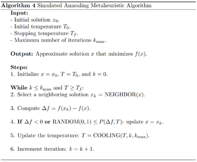
'''Simulated Annealing (SA)''' is a probabilistic optimization technique inspired by the annealing process in metallurgy, where controlled cooling of a material allows it to reach a minimum energy state. This algorithm was introduced by Kirkpatrick, Gelatt, and Vecchi in 1983 as a metaheuristic for solving global optimization problems. SA is particularly effective for complex issues with numerous local optima. The algorithm explores the solution space by accepting improvements and, with decreasing probability, worse solutions to escape local minima. This acceptance probability decreases over time according to a predefined cooling schedule, balancing exploration and exploitation. Due to its simplicity and robustness, SA has been successfully applied across various domains, including combinatorial optimization, scheduling, and machine learning.<ref>Delahaye, D., Chaimatanan, S., Mongeau, M. (2019). Simulated Annealing: From Basics to Applications. In: Gendreau, M., Potvin, JY. (eds) Handbook of Metaheuristics. International Series in Operations Research & Management Science, vol 272. Springer, Cham. https://doi.org/10.1007/978-3-319-91086-4_1. </ref> | '''Simulated Annealing (SA)''' is a probabilistic optimization technique inspired by the annealing process in metallurgy, where controlled cooling of a material allows it to reach a minimum energy state. This algorithm was introduced by Kirkpatrick, Gelatt, and Vecchi in 1983 as a metaheuristic for solving global optimization problems. SA is particularly effective for complex issues with numerous local optima. The algorithm explores the solution space by accepting improvements and, with decreasing probability, worse solutions to escape local minima. This acceptance probability decreases over time according to a predefined cooling schedule, balancing exploration and exploitation. Due to its simplicity and robustness, SA has been successfully applied across various domains, including combinatorial optimization, scheduling, and machine learning.<ref>Delahaye, D., Chaimatanan, S., Mongeau, M. (2019). Simulated Annealing: From Basics to Applications. In: Gendreau, M., Potvin, JY. (eds) Handbook of Metaheuristics. International Series in Operations Research & Management Science, vol 272. Springer, Cham. https://doi.org/10.1007/978-3-319-91086-4_1. </ref> | ||
[[File:Screenshot 2024-12-14 | [[File:Screenshot 2024-12-14 213250.png|center|thumb|400x400px|Figure 5. Simulated Annealing Algorithm Steps]] | ||
''' | == Numerical Example: '''Traveling Salesman Problem (TSP)''' == | ||
The table below show the distance between 4 cities. The algorithm aims to find a near-optimal path that visits all cities exactly once and returns to the starting city with minimal total distance. | |||
{| class="wikitable" | {| class="wikitable" | ||
|+ | |+Distance Matrix | ||
! | ! | ||
Product (i) | Product (i) | ||
| Line 85: | Line 75: | ||
|0.5 | |0.5 | ||
|} | |} | ||
'''( | '''<big><u>Simple Heuristic Algorithms: Greedy Algorithm</u></big>''' | ||
'''Overview:''' | |||
1) Start at any city (A). | |||
2) At each step, move to the '''nearest unvisited city'''. | |||
3) Repeat until all cities are visited. | |||
4) Return to the starting city. | |||
'''Step-by-Step Solution:''' | |||
* '''Start at City A:''' | |||
Unvisited: {B,C,D} | |||
Minimal Distance: A → B (distance = 10) | |||
Path: A → B | |||
Total distance: 10 | |||
* '''Move to City B:''' | |||
Unvisited: {C,D} | |||
Minimal Distance: B → D (distance = 25) | |||
Path: A → B → D | |||
Total distance: 35 | |||
* '''Move to City D:''' | |||
Unvisited: {C} | |||
Minimal Distance: D → C (distance = 30) | |||
Path: A → B → D → C | |||
Total distance: 65 | |||
* '''Return to City A:''' | |||
Path: A → B → D → C → A | |||
Total distance: 80 | |||
'''The greedy algorithm gives us a feasible solution quickly by choosing the nearest neighbor at each step. While it doesn't always guarantee the optimal solution, it's computationally efficient and provides a good starting point for more complex algorithms.''' | |||
'''<big><u>Meta-Heuristic Algorithms: Tabu Search</u></big>''' | |||
'''Overview:''' | |||
1) Generating '''neighborhood solutions'''. | |||
2) Selecting the best neighbor that is not in the '''Tabu List'''. | |||
3) Updating the '''Tabu List''' to prevent cycling. | |||
4) Repeating until a stopping criterion is met. | |||
'''Step-by-Step Solution:''' | |||
* '''Initialization:''' | |||
Initial Path: A → B → C → D → A | |||
Initial Distance: d = 10 + 35 + 30 + 20 = 95 | |||
Tabu List: [ ] (empty) | |||
* '''Generating neighborhood solutions:''' | |||
Neighborhood solutions are created by swapping the order of two cities in the current path (excluding A, the starting city). For the initial path A→B→C→D→A, the possible swaps are: | |||
1. Swap B and C d = 95 | |||
2. Swap B and D d = 95 | |||
3. Swap C and D d = 80 (Best) | |||
* '''Select the best Neighbor that not in the Tabu List''' | |||
Swap C and D is the best Neighbor solution | |||
New Tabu List: [(C,D)] | |||
* '''Repeat Process:''' | |||
New Path: A → B → D → C → A | |||
New Distance: 80 | |||
Tabu List: [(C,D)] | |||
''' | * '''Generating neighborhood solutions''' | ||
Notice (C,D) is in Tabu List, so swapping C and D is not a viable option here. | |||
1. Swap B and C d = 80 (Best) | |||
2. Swap B and D d = 95 | |||
''' | * '''Select the best Neighbor that not in the Tabu List''' | ||
1. Swap B and C is the best Neighbor solution | |||
2. New Tabu List: [(C,D), (B,C)] | |||
… | |||
'''By using a Tabu List, Tabu Search avoids revisiting the same solutions and explores the solution space systematically, and reach the final solution which is 80.''' | |||
<big>'''<u>Simplified approach: Hill Climbing</u>'''</big> | |||
The tabu list above has two impacts on the algorithm. First, it prevents the algorithm from making any choice already chosen, which leads into cycling. Second, it makes the algorithms "flexible" to not always choose the optimal neighborhood solution, which allow exploring the suboptimal space. It is suitable for large and complex problems, but it is more computationally intensive and requires careful parameter tuning. For small and scalable problem, '''Hill Climbing''' is a simpler version. | |||
'''Overview:''' | |||
1) Generating '''neighborhood solutions'''. | |||
2) Selecting the best neighbor that '''improves the objective'''. If there's none, terminate. | |||
3) Repeating until a stopping criterion is met. | |||
'''Notice the process will stop if the current choice is better than any neighborhood solution, which means it will often get stuck in local optima and cannot escape.''' | |||
==Applications== | ==Applications== | ||
Heuristic algorithms | Heuristic algorithms are extensively applied to optimize processes and solve computationally problems in IT field. They are used in network design and routing, where algorithms like A-star and Dijkstra help determine the most efficient paths for data transmission in communication networks. Cloud computing benefits from heuristics for resource allocation and load balancing, ensuring optimal distribution of tasks.<ref>Guo, Lizheng, et al. "Task scheduling optimization in cloud computing based on heuristic algorithm." ''Journal of networks'' 7.3 (2012): 547.</ref> Moreover, heuristic algorithms also thrive in numerous domains. In biology, heuristics approaches, like asBLAST and FASTA, are used to solve problems such as DNA and specific protein comparing.<ref>Chauhan, Shubhendra Singh, and Shikha Mittal. "Exact, Heuristics and Other Algorithms in Computational Biology." ''Bioinformatics and Computational Biology''. Chapman and Hall/CRC, 2023. 38-51.</ref> Heuristic algorithms are also instrumental in finance, optimizing the portfolios to balance risk and payback. <ref>Gilli, Manfred, Dietmar Maringer, and Peter Winker. "Applications of heuristics in finance." ''Handbook on information technology in finance'' (2008): 635-653.</ref> | ||
==Conclusion== | ==Conclusion== | ||
Heuristic algorithms are | Heuristic algorithms are widely applied in solving complex optimization problems where finding an exact solution is computationally infeasible. These algorithms use problem-specific strategies to explore the solution space efficiently, often arriving at near-optimal solutions in a fraction of the time required by exact methods. While heuristic algorithms may not always guarantee the optimal solution, their efficiency, scalability, and flexibility make them an important tool for those challenges in real world. These options allow us to make a call of compromise between computational feasibility and solution quality. As technology advances and problems grow in complexity, heuristic algorithms will continue to evolve to delve and improvise more potential in optimization. | ||
==References== | ==References== | ||
<references /> | <references /> | ||
Latest revision as of 18:44, 15 December 2024
Author: Zemin Mi (zm287), Boyu Yang (by274) (ChemE 6800 Fall 2024)
Stewards: Nathan Preuss, Wei-Han Chen, Tianqi Xiao, Guoqing Hu
Introduction
Heuristic algorithms are strategies designed to efficiently tackle complex optimization problems by providing approximate solutions when exact methods are impractical. This approach is particularly beneficial in scenarios where traditional algorithms may be computationally prohibitive.[1] Heuristics are widely used because they excel in handling uncertainty, incomplete information, and large-scale optimization tasks. Their adaptability, scalability, and integration with other techniques make them valuable across fields like artificial intelligence, logistics, and operations research. Balancing speed and solution quality makes heuristics indispensable for tackling real-world challenges where optimal solutions are often infeasible.[2] A prominent category within heuristic methods is metaheuristics, which are higher-level strategies that effectively guide the search process to explore the solution space. These include genetic algorithms, simulated annealing, and particle swarm optimization. Metaheuristics are designed to balance exploration and exploitation, thereby enhancing the likelihood of identifying near-optimal solutions across diverse problem domains.[3]
Methodology & Classic Example
Optimization heuristics can be categorized into two broad classes based on their approach, focus, and application: heuristics and metaheuristics.
Heuristics
Heuristics are problem-solving methods that employ practical techniques to produce satisfactory solutions within a reasonable timeframe, especially when exact methods are impractical due to computational constraints. These algorithms utilize rules of thumb, educated guesses, and intuitive judgments to navigate complex search spaces efficiently. By focusing on the most promising areas of the search space, heuristics can quickly find good enough solutions without guaranteeing optimality.[4]
Metaheuristics
Metaheuristics are high-level optimization strategies designed to efficiently explore large and complex search spaces to find near-optimal solutions for challenging problems. They guide subordinate heuristics using concepts derived from artificial intelligence, biology, mathematics, and physical sciences to enhance performance.[5] Unlike problem-specific algorithms, metaheuristics are flexible and can be applied across various domains, making them valuable tools for solving real-world optimization challenges. By balancing the global search space exploration with the exploitation of promising local regions, metaheuristics effectively navigate complex landscapes to identify high-quality solutions.
Classic Example: Traveling Salesman Problem (TSP)
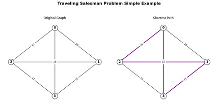
The traveling salesman problem states that given a set of n cities and the distances between each pair of cities, the objective is to find the shortest possible tour that starts and ends in the same city and visits each city exactly once.[6]
- Heuristics solve the TSP by providing efficient and practical approaches to finding approximate solutions, especially for large instances where exact algorithms are computationally infeasible. Instead of exhaustively exploring all possible tours, heuristics focus on simplifying the problem using strategies like incremental solution building, iterative improvement, or probabilistic exploration. For example, constructive heuristics can create a feasible tour by starting at a city and iteratively adding the nearest unvisited city until all cities are covered. To reduce the total travel distance, local search heuristics refine an initial solution by making minor adjustments, such as swapping the order of cities.
- Metaheuristics, such as simulated annealing or genetic algorithms, tackle the TSP by employing high-level strategies to explore the solution space more broadly and escape local optima. These methods balance global search space exploration with local exploitation of promising regions, allowing for a more thorough search for better solutions. They iteratively improve the solution while occasionally considering less favorable configurations to avoid being confined to suboptimal areas. By guiding the search process intelligently, metaheuristics adapt dynamically and effectively solve the TSP, often producing near-optimal solutions even for large-scale or complex problem instances.
Popular Optimization Heuristics Algorithms
Heuristic Algorithms
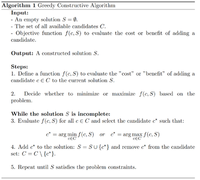
Constructive Algorithm (Greedy)
Constructive heuristics are algorithmic strategies that build solutions incrementally, starting from an empty set and adding elements sequentially until a complete and feasible solution is formed (greedy algorithms). This approach is particularly advantageous due to its simplicity in design, analysis, implementation and limited computational complexity. However, the quality of solutions produced by constructive heuristics heavily depends on the criteria used for adding elements, and they may only sometimes yield optimal results.[7]
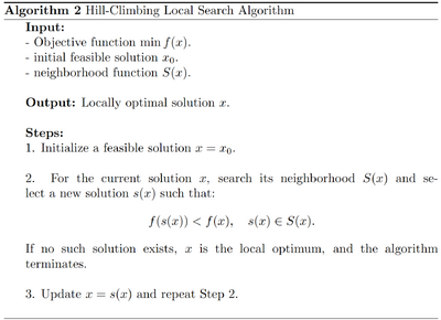
Local Search Algorithm (Hill-Climbing)
Local search heuristics are optimization techniques that iteratively refine a single solution by exploring its immediate neighborhood to find improved solutions. Starting from an initial solution, these methods make incremental changes to enhance the objective function with each iteration. This approach is particularly effective for complex combinatorial problems where an exhaustive search is impractical. However, local search heuristics can become trapped in local optima, focusing on immediate improvements without considering the global solution space. Various strategies, such as random restarts or memory-based enhancements, are employed to escape local optima and explore the solution space more broadly.[8]
Metaheuristic Algorithms
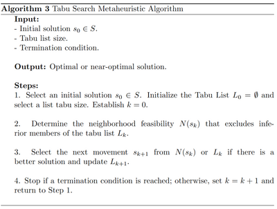
Tabu Search Algorithm
Tabu Search (TS) is an advanced metaheuristic optimization technique designed to navigate complex search spaces and escape local optima using adaptive memory structures. Introduced by Fred Glover in 1986, TS systematically explores neighborhoods of solutions, employing a tabu list to record recently visited solutions or attributes, thereby preventing the search from cycling back to them. This strategic use of memory enables TS to traverse regions of the solution space that traditional local search methods might overlook, enhancing its capability to find near-optimal solutions across various combinatorial optimization problems.[9]
Simulated Annealing Algorithm
Simulated Annealing (SA) is a probabilistic optimization technique inspired by the annealing process in metallurgy, where controlled cooling of a material allows it to reach a minimum energy state. This algorithm was introduced by Kirkpatrick, Gelatt, and Vecchi in 1983 as a metaheuristic for solving global optimization problems. SA is particularly effective for complex issues with numerous local optima. The algorithm explores the solution space by accepting improvements and, with decreasing probability, worse solutions to escape local minima. This acceptance probability decreases over time according to a predefined cooling schedule, balancing exploration and exploitation. Due to its simplicity and robustness, SA has been successfully applied across various domains, including combinatorial optimization, scheduling, and machine learning.[10]
Numerical Example: Traveling Salesman Problem (TSP)
The table below show the distance between 4 cities. The algorithm aims to find a near-optimal path that visits all cities exactly once and returns to the starting city with minimal total distance.
|
Product (i) |
Weight per unit (wi) | Value per unit (vi) |
|---|---|---|
| 1 | 7 | 9 |
| 2 | 5 | 4 |
| 3 | 4 | 3 |
| 4 | 3 | 2 |
| 5 | 1 | 0.5 |
Simple Heuristic Algorithms: Greedy Algorithm
Overview:
1) Start at any city (A).
2) At each step, move to the nearest unvisited city.
3) Repeat until all cities are visited.
4) Return to the starting city.
Step-by-Step Solution:
- Start at City A:
Unvisited: {B,C,D}
Minimal Distance: A → B (distance = 10)
Path: A → B
Total distance: 10
- Move to City B:
Unvisited: {C,D}
Minimal Distance: B → D (distance = 25)
Path: A → B → D
Total distance: 35
- Move to City D:
Unvisited: {C}
Minimal Distance: D → C (distance = 30)
Path: A → B → D → C
Total distance: 65
- Return to City A:
Path: A → B → D → C → A
Total distance: 80
The greedy algorithm gives us a feasible solution quickly by choosing the nearest neighbor at each step. While it doesn't always guarantee the optimal solution, it's computationally efficient and provides a good starting point for more complex algorithms.
Meta-Heuristic Algorithms: Tabu Search
Overview:
1) Generating neighborhood solutions.
2) Selecting the best neighbor that is not in the Tabu List.
3) Updating the Tabu List to prevent cycling.
4) Repeating until a stopping criterion is met.
Step-by-Step Solution:
- Initialization:
Initial Path: A → B → C → D → A
Initial Distance: d = 10 + 35 + 30 + 20 = 95
Tabu List: [ ] (empty)
- Generating neighborhood solutions:
Neighborhood solutions are created by swapping the order of two cities in the current path (excluding A, the starting city). For the initial path A→B→C→D→A, the possible swaps are:
1. Swap B and C d = 95
2. Swap B and D d = 95
3. Swap C and D d = 80 (Best)
- Select the best Neighbor that not in the Tabu List
Swap C and D is the best Neighbor solution
New Tabu List: [(C,D)]
- Repeat Process:
New Path: A → B → D → C → A
New Distance: 80
Tabu List: [(C,D)]
- Generating neighborhood solutions
Notice (C,D) is in Tabu List, so swapping C and D is not a viable option here.
1. Swap B and C d = 80 (Best)
2. Swap B and D d = 95
- Select the best Neighbor that not in the Tabu List
1. Swap B and C is the best Neighbor solution
2. New Tabu List: [(C,D), (B,C)]
…
By using a Tabu List, Tabu Search avoids revisiting the same solutions and explores the solution space systematically, and reach the final solution which is 80.
Simplified approach: Hill Climbing
The tabu list above has two impacts on the algorithm. First, it prevents the algorithm from making any choice already chosen, which leads into cycling. Second, it makes the algorithms "flexible" to not always choose the optimal neighborhood solution, which allow exploring the suboptimal space. It is suitable for large and complex problems, but it is more computationally intensive and requires careful parameter tuning. For small and scalable problem, Hill Climbing is a simpler version.
Overview:
1) Generating neighborhood solutions.
2) Selecting the best neighbor that improves the objective. If there's none, terminate.
3) Repeating until a stopping criterion is met.
Notice the process will stop if the current choice is better than any neighborhood solution, which means it will often get stuck in local optima and cannot escape.
Applications
Heuristic algorithms are extensively applied to optimize processes and solve computationally problems in IT field. They are used in network design and routing, where algorithms like A-star and Dijkstra help determine the most efficient paths for data transmission in communication networks. Cloud computing benefits from heuristics for resource allocation and load balancing, ensuring optimal distribution of tasks.[11] Moreover, heuristic algorithms also thrive in numerous domains. In biology, heuristics approaches, like asBLAST and FASTA, are used to solve problems such as DNA and specific protein comparing.[12] Heuristic algorithms are also instrumental in finance, optimizing the portfolios to balance risk and payback. [13]
Conclusion
Heuristic algorithms are widely applied in solving complex optimization problems where finding an exact solution is computationally infeasible. These algorithms use problem-specific strategies to explore the solution space efficiently, often arriving at near-optimal solutions in a fraction of the time required by exact methods. While heuristic algorithms may not always guarantee the optimal solution, their efficiency, scalability, and flexibility make them an important tool for those challenges in real world. These options allow us to make a call of compromise between computational feasibility and solution quality. As technology advances and problems grow in complexity, heuristic algorithms will continue to evolve to delve and improvise more potential in optimization.
References
- ↑ Kokash, N. (2008). An introduction to heuristic algorithms. Department of Informatics and Telecommunications (2005): pages 1-8. https://www.researchgate.net/publication/228573156.
- ↑ Ezugwu, A.E., Shukla, A.K., Nath, R. et al. (2021). Metaheuristics: a comprehensive overview and classification along with bibliometric analysis. Artif Intell Rev 54, 4237–4316. https://doi.org/10.1007/s10462-020-09952-0.
- ↑ Salhi, S., Thompson, J. (2022). An Overview of Heuristics and Metaheuristics. In: Salhi, S., Boylan, J. (eds) The Palgrave Handbook of Operations Research. Palgrave Macmillan, Cham. https://doi.org/10.1007/978-3-030-96935-6_11.
- ↑ Silver, E. (2004). An overview of heuristic solution methods. J Oper Res Soc 55, 936–956. https://doi.org/10.1057/palgrave.jors.2601758.
- ↑ Osman, I.H., Kelly, J.P. (1996). Meta-Heuristics: An Overview. In: Osman, I.H., Kelly, J.P. (eds) Meta-Heuristics. Springer, Boston, MA. https://doi.org/10.1007/978-1-4613-1361-8_1.
- ↑ Xiao, N. (2009). Evolutionary Algorithms, International Encyclopedia of Human Geography, Elsevier, Pages 660-665. https://doi.org/10.1016/B978-008044910-4.00525-3.
- ↑ Aringhieri, R., Cordone, R., Guastalla, A., Grosso, A. (2023). Constructive and Destructive Methods in Heuristic Search. In: Martí, R., Martínez-Gavara, A. (eds) Discrete Diversity and Dispersion Maximization. Springer Optimization and Its Applications, vol 204. Springer, Cham. https://doi.org/10.1007/978-3-031-38310-6_4.
- ↑ Michiels, W., Aarts, E.H.L., Korst, J. (2018). Theory of Local Search. In: Martí, R., Pardalos, P., Resende, M. (eds) Handbook of Heuristics. Springer, Cham. https://doi.org/10.1007/978-3-319-07124-4_6.
- ↑ Glover, F., Laguna, M. (1998). Tabu Search. In: Du, DZ., Pardalos, P.M. (eds) Handbook of Combinatorial Optimization. Springer, Boston, MA. https://doi.org/10.1007/978-1-4613-0303-9_33.
- ↑ Delahaye, D., Chaimatanan, S., Mongeau, M. (2019). Simulated Annealing: From Basics to Applications. In: Gendreau, M., Potvin, JY. (eds) Handbook of Metaheuristics. International Series in Operations Research & Management Science, vol 272. Springer, Cham. https://doi.org/10.1007/978-3-319-91086-4_1.
- ↑ Guo, Lizheng, et al. "Task scheduling optimization in cloud computing based on heuristic algorithm." Journal of networks 7.3 (2012): 547.
- ↑ Chauhan, Shubhendra Singh, and Shikha Mittal. "Exact, Heuristics and Other Algorithms in Computational Biology." Bioinformatics and Computational Biology. Chapman and Hall/CRC, 2023. 38-51.
- ↑ Gilli, Manfred, Dietmar Maringer, and Peter Winker. "Applications of heuristics in finance." Handbook on information technology in finance (2008): 635-653.