Simplex algorithm

Author: Guoqing Hu (SysEn 6800 Fall 2020)

Steward: Allen Yang, Fengqi You

Introduction

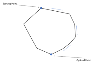
Simplex algorithm (or Simplex method) is a widely-used algorithm to solve the Linear Programming(LP). Simplex algorithm can be thought as one of the elementary steps for solving the inequality problem, since many of those will be converted to LP and solved via Simplex algorithm^[1]. Simplex algorithm has been proposed by George Dantzig, initiated from the idea of step by step downgrade to one of the vortices on the convex polyhedral^[2]. "Simplex" could be possibly referred as the top vertex on the simplicial cone which is the geometric illustration of the constraints within Linear Problem^[3].

Algorithmic Discussion

There are two theorem in LP:

1. The feasible region for any LP problem is a convex set (Every linear equation's second derivative is 0, implying the monotonicity of the trend). Therefore, if an LP has an optimal solution, there must be an extreme point of the feasible region that is optimal
2. For any LP, there is only one extreme point of the LP's feasible region regarding to every basic feasible solution. Plus, there will be at minimum of one basic feasible solution corresponding to every extreme point in the feasible region.^[4]

Geometric Illustration of LP problem

Based on two theorems above, the geometric illustration of the LP problem could be depicted. Each line of this polyhedral will be the boundary of the LP constraints, in which every vertex will be the extreme points according to the theorem. Simplex method is the way to reasonably sort out the shortest path to the optimal solutions.

Consider the following expression as the general linear programming problem standard form:

$\min \sum _{i=1}^{n}c_{i}x_{i}$

With the following constraints:

${\begin{aligned}s.t.\quad \sum _{j=1}^{n}a_{ij}x_{j}&\leq b_{i}\quad i=1,2,...,m\\x_{j}&\geq 0\quad j=1,2,...,n\end{aligned}}$

The first step of the simplex method is to add slack variables and symbols which represent the objective functions:

${\begin{aligned}\phi &=\sum _{i=1}^{n}c_{n}x_{n}\\z_{i}&=b_{i}-\sum _{j=1}^{n}a_{ij}x_{j}\quad i=1,2,...,m\end{aligned}}$

The new introduced slack variables may be confused with the original values. Therefore, it will be convenient to add those slack variables to the end of the list of x-variables with the following expression:

${\begin{aligned}\phi &=\sum _{j=1}^{n}c_{n}x_{n}\\x_{n+i}&=b_{i}-\sum _{j=1}^{n}a_{ij}x_{ij}\quad i=1,2,...,m\end{aligned}}$

With the progression of simplex method, the starting dictionary (which is the equations above) switches between the dictionaries in seeking for optimal values. Every dictionary will have "m" basic variables which form the feasible area, as well as "n" non-basic variables which compose the objective function. Afterward, the dictionary function will be written in the form of:

${\begin{aligned}\phi &={\bar {\phi }}+\sum _{j=1}^{n}{\bar {c_{n}}}x_{n}\\x_{n+i}&={\bar {b_{i}}}-\sum _{j=1}^{n}{\bar {a_{ij}}}x_{ij}\quad i=n+1,n+2,...,n+m\end{aligned}}$

Where pars suggest that those corresponding values will change accordingly with the progression of simplex method. The observation could be made that the basic variables will