Quadratic assignment problem: Difference between revisions

Revision as of 19:02, 21 November 2020

Author: Thomas Kueny, Eric Miller, Natasha Rice, Joseph Szczerba, David Wittmann (SysEn 5800 Fall 2020)

Introduction

Theory, Methodology, and/or Algorithmic Discussions

Joe Szczerba and Tom Kueny to provide.

Numerical Example

Consider the QAP of placing 3 facilities in 3 locations. Let the distance and flow matrices be defined respectively as $D={\begin{bmatrix}0&5&6\\5&0&3.6\\6&3.6&0\end{bmatrix}}$ , ${\textstyle F={\begin{bmatrix}0&10&3\\10&0&6.5\\3&6.5&0\end{bmatrix}}}$ .

For each pair $(i,j)$ , $D_{i,j}$ represents the distance between locations $i$ and $j$ . $F_{i,j}$ represents the required flow (of supplies, products, etc.) between facilities $i$ and $j$ . The optimal solution will be the arrangement of the 3 facilities in the 3 locations so that the total flow over distance is minimized. Intuitively, the product of distance and flow represents cost, and the objective is to minimize this cost. Ideally, two facilities with lots of flow (more product or supplies) between the two should be placed closer together than two facilities that rarely interact (low flow).

There are $3!=6$ permutations of the 3 facilities in the 3 locations. The set of these permutations is typically denoted $S_{3}$ . As an example, the permutation $\phi =(321)$ represents facility 3 being placed at location 1, facility 1 at location 2 and facility 2 at location 3. Each permutation can be assigned a permutation matrix. The permutation matrix of $\phi$ can be written as $X_{\phi }={\begin{bmatrix}0&0&1\\1&0&0\\0&1&0\end{bmatrix}}$ . The operation $X_{\phi }DX_{\phi }^{T}$ permutes the distance matrix values so that $(X_{\phi }DX_{\phi }^{T})_{i,j}$ represents the distance between facilities $i$ and $j$ if the facilities are arranged according to the permutation $\phi$ . Then the cost function between facilities $i$ and $j$ , after being permuted to their location, is $F_{i,j}$ $(X_{\phi }DX_{\phi }^{T})_{i,j}$ . To find the total cost, sum over each $i$ and $j$ for the facilities arranged according to $\phi$ .

Defining the inner product of two matrices $A,B$ as $<A,B>=\sum _{i=1}^{n}\sum _{j=1}^{n}a_{i,j}b_{i,j}$ , the objective function can be written as $<F,XDX^{T}>$ . (Since this matrix is symmetric, and the inner product double counts each value, the optimal cost value will actually requiring dividing by 2).

Let $P$ be the set of permutation matrices for $S_{3}$ . The problem can be stated as follows:

$\min _{X\in P}<F,XDX^{T}>$ . The table lists the resulting cost function to place the facilities according to each permutation $\phi \in S_{3}$ . Note that $\phi =()$ is the identity mapping where the number of the facility is the location number.

Cost for Each Permutation in $S_{3}$
Permutation	Cost
$\phi _{1}=$ ( )	91.4
$\phi _{2}=(12)$	99.8
$\phi _{3}=(23)$	98.4
$\phi _{4}=(13)$	86.5
$\phi _{5}=(123)$	103.3
$\phi _{6}=(132)$	90

Based on these results, $\phi _{4}=(13)$ is the arrangement of facilities that minimizes the cost function with a value of 86.5. Facility 1 should be placed at location 3, Facility 2 remains at location 2 and Facility 3 is placed at location 1.

Applications

Natasha Rice and David Wittmann to provide.

Inter-plant Transportation Problem

The quadratic assignment problem was first introduced by Koopmans and Beckmann to address how economic decisions could be made to optimize the transportation costs of goods between both manufacturing plants and locations. Factoring in the location of the each of the manufacturing plants as well as the volume of goods between locations to maximize revenue is what distinguishes this from other linear programming assignment problems like the Knapsack Problem.

The Backboard Wiring Problem

As the quadratic assignment problem is focused on minimizing the cost of traveling from one location to another, it is an ideal approach determining placement of components in many modern electronics. Leon Steinberg proposed a QAP solution optimize the layout of elements on a blackboard by minimizing the total amount of wiring required.

When defining the problem Steinberg states that we have a set of n elements

$E=\left\{E_{1},E_{2},...,E_{n}\right\}$

as well as a set of r points

$P_{1},P_{2},...,P_{r}$ where $r\geq n$

In his paper he derives the below formula:

$min\sum _{1\leq i\leq j\leq n}^{}C_{ij}(d_{s(i)s(j))})$

$C_{ij}$ represents the number of wires connecting components $E_{i}$ and $E_{i}$

$d_{s(i)s(j))}$ is the length of wire needed to connect tow components if one is placed at $P_{\alpha }$ and the other is placed at $P_{\beta }$ . If $P_{\alpha }$ has coordinates $(x_{\alpha },y_{\alpha },z_{\alpha })$ then $d_{s(i)s(j))}$ can be calculated by

$d_{s(i)s(j))}=\surd ({\bigl (}x_{\alpha }-x_{\beta }{\bigr )}^{2}+{\bigl (}y_{\alpha }-y_{\beta }{\bigr )}^{2}+{\bigl (}z_{\alpha }-z_{\beta }{\bigr )}^{2})$

$s(x)$ represents a particular placement of a component.

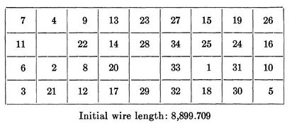
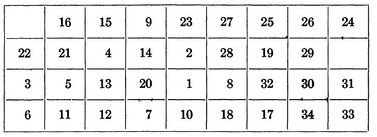
In his paper Steinberg a backboard with a 9 by 4 array, allowing for 36 potential positions for the 34 components that needed to be placed on the backboard. For the calculation he selected a random initial placement of s1 and chose a random family of 25 unconnected sets.

The initial placement of components is shown below:

After the initial placement of elements it took an additional 35 iterations to get us to our final optimized backboard layout. Leading to a total of 59 iterations and a final wire length of 4,969.440.

Hospital Layout

Building a new hospitals was a common event in 1977 when Alealid N Elshafei wrote his paper on "Hospital Layouts as a Quadratic Assignment Problem". With high initial cost to construct the hospital and to staff it, it is important to ensure that it is operating as efficiently as possible. Elshafei's paper was commissioned to create a optimization formula to locate clinics within a building in such a way that minimizes the total distance that a patient travels within the hospital throughout the year. When doing a study of a major hospital in Cario he determined that the Out-patient ward was acting as a bottle neck in the hospital and focused his efforts on optimizing the 17 departments there.

Elshafei identified the following QAP to determine where clinics should be placed:

$min\sum _{i,j}\sum _{k,q}f_{ik}d_{jq}y_{ij}y_{kq}$

Such that $\sum _{j\epsilon J}y_{ij}=1\forall i\epsilon I$

$\sum _{i\epsilon I}y_{ij}=1\forall j\epsilon J$

$y_{ij}{\begin{Bmatrix}1iffacilityiislocatedatj\\0otherwise\end{Bmatrix}}$

$f_{ik}$ is the yearly flow between facilities i and k

$d_{jq}$ is the distance between the possible facility locations j and q

$I$ is the initial set of facilities

$J$ is the initial set of all locations

It can take a large amount of computational power to calculate the solution to a QAP problem, necessitating

Conclusion

References

Alwalid N. Elshafei. Hospital Layout as a Quadratic Assignment Problem. Operational Research Quarterly (1970-1977). 1977;28(1):167. doi:10.2307/3008789
Leon Steinberg. The Backboard Wiring Problem: A Placement Algorithm. SIAM Review. 1961;3(1):37.
https://citeseerx.ist.psu.edu/viewdoc/download?doi=10.1.1.217.1914&rep=rep1&type=pdf
Koopmans, T., & Beckmann, M. (1957). Assignment Problems and the Location of Economic Activities. Econometrica, 25(1), 53-76. doi:10.2307/1907742

@@ Line 17: / Line 17: @@
 There are <math>3! = 6</math> permutations of the 3 facilities in the 3 locations. The set of these permutations is typically denoted <math>S_3 </math>.  As an example, the permutation <math>\phi=(3 2 1)</math> represents facility 3 being placed at location 1, facility 1 at location 2 and facility 2 at location 3. Each permutation can be assigned a permutation matrix. The permutation matrix of <math>\phi </math> can be written as <math>X_{\phi} = \begin{bmatrix} 0 & 0 & 1 \\ 1 & 0 &0 \\ 0 &1 & 0 \end{bmatrix}</math>. The operation <math>X_{\phi}DX_{\phi}^{T} </math> permutes the distance matrix values so that <math>(X_{\phi}DX_{\phi}^{T})_{i,j} </math> represents the distance between facilities <math>i</math> and <math>j</math> if the facilities are arranged according to the permutation <math>\phi</math>. Then the cost function between facilities <math>i</math> and <math>j</math>, after being permuted to their location, is <math>F_{i,j}</math><math>(X_{\phi}DX_{\phi}^{T})_{i,j} </math>. To find the total cost, sum over each <math>i</math> and <math>j</math> for the facilities arranged according to <math>\phi</math>.
 Defining the inner product of two matrices <math>A,B</math> as <math><A,B> = \sum_{i=1}^{n}\sum_{j=1}^{n}a_{i,j}b_{i,j}</math>, the objective function can be written as <math><F,XDX^{T}></math>. (Since this matrix is symmetric, and the inner product double counts each value, the optimal cost value will actually requiring dividing by 2).
-Let <math>P</math> be the set of permutation matrices for <math>S_3 </math>.The problem can be stated as follows:
+Let <math>P</math> be the set of permutation matrices for <math>S_3 </math>. The problem can be stated as follows:
-<math>\min_{X \in P} <F,XDX^{T}></math>
+<math>\min_{X \in P} <F,XDX^{T}></math>. The table lists the resulting cost function to place the facilities according to each permutation <math>\phi \in S_3 </math>. Note that <math>\phi = () </math> is the identity mapping where the number of the facility is the location number.
-{| class="wikitable"
+{| class="wikitable sortable"
-|+<math>S_3</math>
+|+Cost for Each Permutation in <math>S_3 </math>
 |Permutation
 |Cost
-|
-|
 |-
 |<math>\phi_1=</math> ( )
-|
+|91.4
-|
-|
 |-
 |<math>\phi_2= (1 2)</math>
-|
+|99.8
-|
-|
 |-
 |<math>\phi_3=(23)</math>
-|
+|98.4
-|
-|
 |-
 |<math>\phi_4=(13)</math>
-|
+|86.5
-|
-|
 |-
 |<math>\phi_5=(123)</math>
-|
+|103.3
-|
-|
 |-
 |<math>\phi_6=(132)</math>
-|
+|90
-|
-|
 |}
+Based on these results, <math>\phi_4=(13)</math> is the arrangement of facilities that minimizes the cost function with a value of 86.5. Facility 1 should be placed at location 3, Facility 2 remains at location 2 and Facility 3 is placed at location 1.
 == Applications ==