Markov decision process: Difference between revisions
No edit summary |
|||
| Line 45: | Line 45: | ||
</math> | </math> | ||
The value function can be decomposed into two parts, the immediate reward of the current state, and the discounted value of the next state. This decomposition leads to the derivation of the [[Bellman equation|Bellman Equation]] | The value function can be decomposed into two parts, the immediate reward of the current state, and the discounted value of the next state. This decomposition leads to the derivation of the [[Bellman equation|Bellman Equation]]. Because the actions and rewards are dependent on the policy, the value function of an MDP is associated with a given policy. | ||
<math>v(s) = E[ r_{t+1} + \gamma v(s_{t+1}) | s_t] | <math>v(s) = E[ r_{t+1} + \gamma v(s_{t+1}) | s_t] | ||
| Line 51: | Line 51: | ||
<math>v(s) = R(s) + \gamma \sum_{s' \epsilon S}P_{ss'}V(s') | <math>v(s) = R(s) + \gamma \sum_{s' \epsilon S}P_{ss'}V(s') | ||
</math> | |||
<math>v^{\pi}(s) = R(s,\pi(s)) + \gamma \sum_{s' \epsilon S}P(s' | s,\pi(s))V(s') | |||
</math> | </math> | ||
| Line 63: | Line 66: | ||
</math> | </math> | ||
The policy is a function of the current state, meaning at each time step a new policy is calculated considering the present information. The optimal value function can be solved using methods such as value iteration, policy iteration, or linear programming. | The policy is a function of the current state, meaning at each time step a new policy is calculated considering the present information. The optimal value function can be solved using methods such as value iteration, policy iteration, Q-learning, or linear programming. | ||
'''The Algorithm''' | '''The Algorithm''' | ||
| Line 138: | Line 141: | ||
# Abbeel, P. (n.d.). ''Markov Decision Processes and Exact Solution Methods:'' 34. | # Abbeel, P. (n.d.). ''Markov Decision Processes and Exact Solution Methods:'' 34. | ||
# Ashraf, M. (2018, April 11). ''Reinforcement Learning Demystified: Markov Decision Processes (Part 1)''. Medium. <nowiki>https://towardsdatascience.com/reinforcement-learning-demystified-markov-decision-processes-part-1-bf00dda41690</nowiki> | # Ashraf, M. (2018, April 11). ''Reinforcement Learning Demystified: Markov Decision Processes (Part 1)''. Medium. <nowiki>https://towardsdatascience.com/reinforcement-learning-demystified-markov-decision-processes-part-1-bf00dda41690</nowiki> | ||
# Bertsekas, D. P. ( | # Bertsekas, D. P. (2011). Dynamic Programming and Optimal Control 3rd Edition, Volume II. ''Massachusetts Institue of Technology'', 233. | ||
# Littman, M. L. (2001). Markov Decision Processes. In N. J. Smelser & P. B. Baltes (Eds.), ''International Encyclopedia of the Social & Behavioral Sciences'' (pp. 9240–9242). Pergamon. <nowiki>https://doi.org/10.1016/B0-08-043076-7/00614-8</nowiki> | # Littman, M. L. (2001). Markov Decision Processes. In N. J. Smelser & P. B. Baltes (Eds.), ''International Encyclopedia of the Social & Behavioral Sciences'' (pp. 9240–9242). Pergamon. <nowiki>https://doi.org/10.1016/B0-08-043076-7/00614-8</nowiki> | ||
# Mnih, V., Kavukcuoglu, K., Silver, D., Graves, A., Antonoglou, I., Wierstra, D., & Riedmiller, M. (2013). Playing Atari with Deep Reinforcement Learning. ''ArXiv:1312.5602 [Cs]''. <nowiki>http://arxiv.org/abs/1312.5602</nowiki> | # Mnih, V., Kavukcuoglu, K., Silver, D., Graves, A., Antonoglou, I., Wierstra, D., & Riedmiller, M. (2013). Playing Atari with Deep Reinforcement Learning. ''ArXiv:1312.5602 [Cs]''. <nowiki>http://arxiv.org/abs/1312.5602</nowiki> | ||
Revision as of 23:07, 12 December 2020
Author: Eric Berg (eb645), Fall 2020
Introduction
A Markov Decision Process (MDP) is a stochastic sequential decision making method.$ ^1 $ Sequential decision making is applicable any time there is a dynamic system that is controlled by a decision maker where decisions are made sequentially over time. MDPs can be used to determine what action the decision maker should make given the current state of the system and its environment. This decision making process takes into account information from the environment, actions performed by the agent, and rewards in order to decide the optimal next action. MDPs can be characterized as both finite or infinite and continuous or discrete depending on the set of actions and states available and the decision making frequency.$ ^1 $ This article will focus on discreet MDPs with finite states and finite actions for the sake of simplified calculations and numerical examples. The name Markov refers to the Russian mathematician Andrey Markov, since the Markov Decision Process is based on the Markov Property. In the past, MDPs have been used to solve problems like inventory control, queuing optimization, and routing problems.$ ^2 $ Today, MDPs are often used as a method for decision making in the reinforcement learning applications, serving as the framework guiding the machine to make decisions and "learn" how to behave in order to achieve its goal.
Theory and Methodology
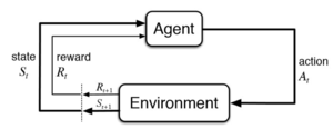
A Markov Decision process makes decisions using information about the system's current state, the actions being performed by the agent and the rewards earned based on states and actions.
The MDP is made up of multiple fundamental elements: the agent, states, a model, actions, rewards, and a policy.$ ^1 $ The agent is the object or system being controlled that has to make decisions and perform actions. The agent lives in an environment that can be described using states, which contain information about the agent and the environment. The model determines the rules of the world in which the agent lives, in other words, how certain states and actions lead to other states. The agent can perform a fixed set of actions in any given state. The agent receives rewards based on its current state. A policy is a function that determines the agent's next action based on its current state.

MDP Framework:
- $ S $ : States ($ s \epsilon S $)
- $ A $ : Actions ($ a \epsilon A $)
- $ P(S_{t+1} | s_t, a_t) $ : Model determining transition probabilities
- $ R(s) $: Reward
In order to understand how the Markov Decision Process works, first the Markov Property must be defined. The Markov Property states that the future is independent of the past given the present. $ ^4 $In other words, only the present is needed to determine the future, since the present contains all necessary information from the past. The Markov Property can be described in mathematical terms below:
$ {\textstyle P[S_{t+1} | S_t] = P[S_{t+1} | S_1, S_2, S_3... S_t]} $
The above notation conveys that the probability of the next state given the current state is equal to the probability of the next state given all previous states. The Markov Property is relevant to the Markov Decision Process because only the current state is used to determine the next action, the previous states and actions are not needed.
The Policy and Value Function
The policy, $ \Pi $ , is a function that maps actions to states. The policy determines which is the optimal action given the current state to achieve the maximum total reward.
$ \Pi : S \rightarrow A $
Before the best policy can be determined, a the goal or return must be defined to quantify rewards at every state. There are various ways to define the return. Each variation of the return function tries to maximize rewards in some way, but differs in which accumulation of rewards should be maximized. The first method is to choose the action that maximizes the expected reward given the current state. This is the myopic method, which weighs each time-step decision equally. Next is the finite-horizon method, which tries to maximize the accumulated reward over a fixed number of time steps. But because many applications may have infinite horizons, meaning the agent will always have to make decisions and continuously try to maximize its reward, another method is commonly used, known as the infinite-horizon method. In the infinite-horizon method, the goal is to maximize the expected sum of rewards over all steps in the future. When performing an infinite sum of rewards that are all weighed equally, the results may not converge and the policy algorithm may get stuck in a loop. In order to avoid this, and to be able prioritize short-term or long term-rewards, a discount factor, $ \gamma $, is added. If $ \gamma $ is closer to 0, the policy will choose actions that prioritize more immediate rewards, and $ \gamma $ is closer to 1, long-term rewards are prioritized.
Return/Goal Variations:
- Myopic: Maximize $ E[ r_t | \Pi , s_t ] $ , maximize expected reward for each state
- Finite-horizon: Maximize $ E[ \textstyle \sum_{t=0}^k \displaystyle r_t | \Pi , s_t ] $
- Discounted Infinite-horizon: Maximize $ E[ \textstyle \sum_{t=0}^\infty \displaystyle \gamma^t r_t | \Pi , s_t ] $ $ \gamma \epsilon [0,1] $
The value function, $ v(s) $, characterizes the return at a given state. Most commonly, the discounted infinite horizon return method is used to determine the best policy. Below the value function is defined as the expected sum of discounted future rewards.
$ v(s) = E[ \sum_{t=0}^\infty \gamma^t r_t | s_t ] $
The value function can be decomposed into two parts, the immediate reward of the current state, and the discounted value of the next state. This decomposition leads to the derivation of the Bellman Equation. Because the actions and rewards are dependent on the policy, the value function of an MDP is associated with a given policy.
$ v(s) = E[ r_{t+1} + \gamma v(s_{t+1}) | s_t] $
$ v(s) = R(s) + \gamma \sum_{s' \epsilon S}P_{ss'}V(s') $
$ v^{\pi}(s) = R(s,\pi(s)) + \gamma \sum_{s' \epsilon S}P(s' | s,\pi(s))V(s') $
The value function can solved iteratively using iterative methods such as dynamic programming, Monte-Carlo evaluations, or temporal-difference learning.
The optimal policy is one that chooses the action with the largest value given the current state:
$ \Pi(s) = max_a [R(s,a) + \gamma \sum_{s' \epsilon S}P_{ss'}^aV(s')] $
$ \Pi(s) = max_{\Pi} V_{\Pi}(s) $
The policy is a function of the current state, meaning at each time step a new policy is calculated considering the present information. The optimal value function can be solved using methods such as value iteration, policy iteration, Q-learning, or linear programming.
The Algorithm
At each step, given state $ s_t $
- Update Value Function $ V(s) $
- Update Policy $ \Pi(s) $ and perform action $ a $
Numerical Example

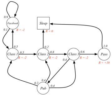
As an example, the Markov decision process can be applied to a college student, depicted to the right. In this case, the agent would be the student. The states would be the circles and squares in the diagram, and the arrows would be the actions. The actions between class states would be "study". In the state that the student is in Class 2, the allowable actions are to study or sleep. The model in this case would assign probabilities to each state given the previous state and action. These probabilities are written next to the arrows. Finally the rewards associated with each state are written in red.
Assume the first state is Class 1, $ \gamma $ =1.
First, the value functions must be calculated for each state.
$ V(s) = R(s) + \gamma \sum_{s' \epsilon S}P_{ss'}V(s') $
$ V(Class 1) = -1.3 $
$ V(Class 2) = 2.7 $
$ V(Sleep) = 0 $
$ V(Pass) = 10 + (1)(1.0*0)=10 $
$ V(Facebook) = -1 + (1)(0.9*-1 + 0.1*-1.3)= -2.03 $
$ V(Class3) = -2 + 1(0.6*10+0.4(0.2*-1.3 +0.4*2.7 +0.4*7.4)) = 7.4 $
Then, in state 1 (Class 1), the optimal policy is that the action chosen should result in the state that generates the highest value function.
$ \Pi(s) = max_a [R(s,a) + \gamma \sum_{s' \epsilon S}P_{ss'}^aV(s')] $
$ \Pi(Class 1) = max_a [-2+2.7,-1-2.03] = max_a [0.7,-3.03] =0.7 $
$ a = $ = study and go to Class 2
Therefore, the optimal policy in state Class 1 is to go to Class 2. Now, the optimal policy action can be decided in each state using the same process.
Applications

Markov Decision Processes have been applied in various fields including operations research, electrical engineering, computer science, manufacturing, economics, finance, and telecommunication.$ ^2 $ For example, the sequential decision making process described by MDP can be used to solve routing problems such as the Traveling salesman problem. In this case, the agent is the salesman, the actions available are the routes available take from the current state, the rewards in this case consists of cost of taking each route, and the goal is to determine the optimal policy that minimizes the cost function over the duration of the trip. Another application example is maintenance and repair problems, in which a dynamic system such as a vehicle will deteriorate over time due to its actions and the environment, and the available decisions at every time epoch is to do nothing, repair, or replace a certain component of the system.$ ^2 $ This problem can be formulated as an MDP to choose the actions that to minimize cost of maintenance over the life of the vehicle. MDPs have also been applied to optimize telecommunication protocols, stock trading, and queue control in manufacturing environments. $ ^2 $
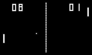
Given the significant advancements in artificial intelligence and machine learning over the past decade, MDPs are being applied in fields such as robotics, automated systems, and autonomous vehicles, and other complex autonomous systems. MDPs have been used widely within reinforcement learning to teach robots or other computer-based systems how to do something they were previously were unable to do. For example, Markov decision processes have been used to teach a computer how to play computer games like Pong, Pacman, or AlphaGo.$ ^{7,8} $ DeepMind Technologies, owned by Google, used the MDP framework in conjunction with neural networks to play Atari games better than human experts. $ ^7 $ In this application, only the raw pixel input of the game screen was used as input, and a neural network was used to estimate the value function for each state, and choose the next action.$ ^7 $ MDPs have been used in more advanced applications to teach a simulated human robot how to walk and run and a real legged-robot how to walk.$ ^9 $

Conclusion
A Markov Decision Process is a stochastic, sequential decision-making method based on the Markov Property. MDPs can be used to make optimal decisions for a dynamic system given information about its current state and its environment. This process is fundamental in reinforcement learning applications and a core method for developing artificially intelligent systems. MDPs have been applied to a wide variety of industries and fields including robotics, operations research, manufacturing, economics, and finance.
References
- Puterman, M. L. (1990). Chapter 8 Markov decision processes. In Handbooks in Operations Research and Management Science (Vol. 2, pp. 331–434). Elsevier. https://doi.org/10.1016/S0927-0507(05)80172-0
- Feinberg, E. A., & Shwartz, A. (2012). Handbook of Markov Decision Processes: Methods and Applications. Springer Science & Business Media.
- Abbeel, P. (n.d.). Markov Decision Processes and Exact Solution Methods: 34.
- Ashraf, M. (2018, April 11). Reinforcement Learning Demystified: Markov Decision Processes (Part 1). Medium. https://towardsdatascience.com/reinforcement-learning-demystified-markov-decision-processes-part-1-bf00dda41690
- Bertsekas, D. P. (2011). Dynamic Programming and Optimal Control 3rd Edition, Volume II. Massachusetts Institue of Technology, 233.
- Littman, M. L. (2001). Markov Decision Processes. In N. J. Smelser & P. B. Baltes (Eds.), International Encyclopedia of the Social & Behavioral Sciences (pp. 9240–9242). Pergamon. https://doi.org/10.1016/B0-08-043076-7/00614-8
- Mnih, V., Kavukcuoglu, K., Silver, D., Graves, A., Antonoglou, I., Wierstra, D., & Riedmiller, M. (2013). Playing Atari with Deep Reinforcement Learning. ArXiv:1312.5602 [Cs]. http://arxiv.org/abs/1312.5602
- Silver, D., Hubert, T., Schrittwieser, J., Antonoglou, I., Lai, M., Guez, A., Lanctot, M., Sifre, L., Kumaran, D., Graepel, T., Lillicrap, T., Simonyan, K., & Hassabis, D. (2018). A general reinforcement learning algorithm that masters chess, shogi, and Go through self-play. Science, 362(6419), 1140–1144. https://doi.org/10.1126/science.aar6404
- Ha, S., Xu, P., Tan, Z., Levine, S., & Tan, J. (2020). Learning to Walk in the Real World with Minimal Human Effort. ArXiv:2002.08550 [Cs]. http://arxiv.org/abs/2002.08550
- Platt, R. (n.d.). Markov Decision Processes. 66.
- Roberts, J. (n.d.). Markov Decision Processes. 24.
- Silver, D. (n.d.). Lecture 2: Markov Decision Processes. Markov Processes, 57.