Job shop scheduling: Difference between revisions
No edit summary |
No edit summary |
||
| Line 51: | Line 51: | ||
There are four jobs that need to be processed on a single shared resource. Each job has a finite duration to complete and a due date in the overall project schedule. This information is shown in the following table: | There are four jobs that need to be processed on a single shared resource. Each job has a finite duration to complete and a due date in the overall project schedule. This information is shown in the following table: | ||
{| class="wikitable" | {| class="wikitable" | ||
|+Job Information | |+Table 1: Job Information | ||
!Job | !Job | ||
!Duration (days) | !Duration (days) | ||
| Line 72: | Line 72: | ||
|Day 14 | |Day 14 | ||
|} | |} | ||
The goal of this method is to determine the order in which the jobs should be processed on the shared resource to minimize total accrued project delay. There are n! feasible solutions for a job shop scheduling problem, therefore there are 4! = 24 feasible solutions for this example. The completion day is the summation of all job durations in a given sequence. The delay per job is found by subtracting a job's due date by the job's calculated completion day. Total project delay is the summation of all individual job delays. The following table shows an example to calculate delay for one particular sequence, ABCD. | The goal of this method is to determine the order in which the jobs should be processed on the shared resource to minimize total accrued project delay. There are n! feasible solutions for a job shop scheduling problem, therefore there are 4! = 24 feasible solutions for this example. The project completion day is the summation of all job durations in a given sequence. The delay per job is found by subtracting a job's due date by the job's calculated completion day. Total project delay is the summation of all individual job delays. The following table shows an example to calculate delay for one particular sequence, ABCD. | ||
{| class="wikitable" | {| class="wikitable" | ||
|+Delay for Sequence (A, B, C, D) | |+Table 2: Delay for Sequence (A, B, C, D) | ||
!Job | !Job | ||
!Completion Day | !Completion Day | ||
| Line 95: | Line 95: | ||
|''d<sub>4</sub> = 24 - 14 = 10'' | |''d<sub>4</sub> = 24 - 14 = 10'' | ||
|} | |} | ||
By beginning with job A at day 0, it will be completed by day 3. This is 2 days before the job A deadline and adds no delay to the overall schedule. At completion of job B we add the 3 days used on job A to the 5 needed for job B to get a completion time of 8 days. This yields a 2 day delay, as the deadline for job B was day 6. Finally we repeat that process for job C and job D yielding an additional 1 and 10 day delay respectively. The total project delay T is equal to the summation of the accrued delay for each | By beginning with job A at day 0, it will be completed by day 3. This is 2 days before the job A deadline and adds no delay to the overall schedule. At completion of job B we add the 3 days used on job A to the 5 needed for job B to get a completion time of 8 days. This yields a 2 day delay, as the deadline for job B was day 6. Finally we repeat that process for job C and job D yielding an additional 1 and 10 day delay respectively. The total project delay T is equal to the summation of the accrued delay for each job: T = ''d<sub>1</sub>'' + ''d<sub>2</sub>'' + ''d<sub>3</sub> + d<sub>4</sub>= 0 + 2 + 1 + 10 = 13 days.'' | ||
Using the Branch and Bound method, we can expand upon this concept and determine the sequence yielding the smallest delay out of all 24 feasible solutions. We first define our decision variables where ''X<sub>ij</sub>'' = 1 if job j is put in the ith position, and ''X<sub>ij</sub>'' = 0 otherwise. Positions of jobs in the sequence are denoted by i = 1, 2, 3, 4; Jobs are denoted by j = A, B, C, D. | Using the Branch and Bound method, we can expand upon this concept and determine the sequence yielding the smallest delay out of all 24 feasible solutions. We first define our decision variables where ''X<sub>ij</sub>'' = 1 if job j is put in the ith position, and ''X<sub>ij</sub>'' = 0 otherwise. Positions of jobs in the sequence are denoted by i = 1, 2, 3, 4; Jobs are denoted by j = A, B, C, D. | ||
Initially, the ideal sequence of the jobs, the delay for any individual job, or the total delay are unknown. | Initially, the ideal sequence of the jobs, the delay for any individual job, or the total project delay are unknown. | ||
[[File:ExampleStep1.png|alt=|none|thumb|329x329px|'''Figure 2:''' Example Step 1 - Optimal position for any job, delay for any job, and total delay are all unknown.]] | [[File:ExampleStep1.png|alt=|none|thumb|329x329px|'''Figure 2:''' Example Step 1 - Optimal position for any job, delay for any job, and total project delay are all unknown.]] | ||
We begin by looking at the final position in the sequence. The completion date for the final job in the sequence is always known, since it is the summation of all | We begin by looking at the final position in the sequence. The completion date for the final job in the sequence is always known, since it is the summation of all job durations that need to be completed. In this example we know the final task will complete on day 24, as seen in table 2 above. Next we can calculate the delay that the final task will have, given it is the last job in the sequence, by subtracting the task due date from 24. After determining which job will yield the smallest delay when in the last position, we branch from that job and repeat the process for the second to last job in the sequence. Job A is due on day 5: 24 - 5 = 19 delay. Job B is due on day 6: 24 - 6 = 18 delay. Job C is due on day 16: 24 - 16 = 8 delay. Job D is due on day 14: 24 - 14 = 10 delay. | ||
[[File:Example2 2.png|none|thumb|433x433px|Figure 3: Example Step 2 - Determine the smallest possible project delay given each job is placed last in the sequence.]] | [[File:Example2 2.png|none|thumb|433x433px|Figure 3: Example Step 2 - Determine the smallest possible project delay given each job is placed last in the sequence.]] | ||
Figure 3 shows that job C in the final position of the sequence yields the smallest possible project delay T. Therefore, we branch from this path and repeat the process for the task in the second to last position. Since job C is selected to be last, and has a duration of 9 days, we know that the second to last job will be completed on day 15. From there we can once again use the known due dates of each task to determine the path with the smallest accrued delay. Job A is due on day 5: 15 - 5 = 10 delay. Job B is due on day 6: 15 - 6 = 9 delay. Job D is due on day 14: 15 - 14 = 1 delay. | Figure 3 shows that job C in the final position of the sequence yields the smallest possible project delay T >= 8. Therefore, we branch from this path and repeat the process for the task in the second to last position. Since job C is selected to be last, and has a duration of 9 days, we know that the second to last job will be completed on day 15. From there we can once again use the known due dates of each task to determine the path with the smallest accrued delay. Job A is due on day 5: 15 - 5 = 10 delay. Job B is due on day 6: 15 - 6 = 9 delay. Job D is due on day 14: 15 - 14 = 1 delay. | ||
[[File:Example3.png|none|thumb|785x785px|'''Figure 4:''' Example Step 3 - Branch from node C and determine which job will yeild the lowest possible delay if run second to last. It is known that this job will complete on day 15 (Time to complete job C subtracted by total time to complete jobs 24-9=15).]] | [[File:Example3.png|none|thumb|785x785px|'''Figure 4:''' Example Step 3 - Branch from node C and determine which job will yeild the lowest possible delay if run second to last. It is known that this job will complete on day 15 (Time to complete job C subtracted by total time to complete jobs 24-9=15).]] | ||
Revision as of 22:27, 14 December 2021
Authors: Carly Cozzolino, Brianna Christiansen, Elaine Vallejos, Michael Sorce, Jeff Visk (SYSEN 5800 Fall 2021)
Introduction
The Job-Shop Scheduling Problem (JSSP) is a widely studied combinatorial, NP-hard optimization problem[1]. The aim of the problem is to find the optimum schedule for allocating shared resources over time to competing activities[2] in order to reduce the overall time needed to complete all activities. As one of the most widely studied combinatorial optimization problems, it is unclear who may have originated the problem in its current form, but studies into the problem seem to stem back to the early 1950s, within research into industrial optimization[3].
Within a JSSP you will have n number of jobs (J1, J2, ..., Jn ), that will need to be completed using a m number shared resources, most commonly denoted as machines (M1, M2, ..., Mm ). Each job will have operations (O) that will need to be completed in a specific order in order for the job to be completed. Operations must be completed at specific machines and require a specific amount of processing time (p) on that machine. Machines are assumed to only be able to process one operation at a time, driving the need to optimize the order in which these operations are completed.[2][4] The goal of the JSSP is to minimize the overall time it takes to complete all n jobs within the problem.
The most obvious real world application of the JSSP is within manufacturing and machining as the parameter description describes. Companies that are able to optimize their machining schedules are able to reduce production time and cost in order to maximize profits, while being able to quickly respond to market demands[3]. Other applications include optimization of computer resources in order to reduce processing time for multiple computer tasks, and within the automation industry, as factories begin to automate more and more process such as transporting materials from different points within the factory.
There are a variety of heuristic methods that can be considered in order to execute tasks to maximize efficiency and minimize costs, including Minimum Completion Time, Duplex, Max-Min, Min-min, Tabu Search, and Genetic Algorithms. Each of these methods have their advantages and disadvantages, weighing the importance of minimizing execution time versus finding the closest to optimal solution.[5]
Theory/Methodology/Algorithms
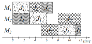
The job shop scheduling problem is NP-hard meaning it’s complexity class for non-deterministic polynomial-time is least as hard as the hardest of problems in NP. As an input, there is a finite set J of jobs and a finite set of M of machines. Some jobs may need to be processed through multiple machines giving us an optimal potential processing order for each job. The processing time of the job j on machine m can be defined as the nonnegative integer . In order to minimize total completion time, the job shop can find the optimal schedule of J on M[6].
These assumptions are required to apply the methods that are discussed to the job shop scheduling problem.
- The number of operations for each job must be finite.
- The processing time for each operation in a particular machine is defined.
- There is a pre-defined sequence of operations that has to be maintained to complete each job.
- Delivery times of the products must be undefined.
- There is no setup cost or tardiness cost.
- A machine can process only one job at a time.
- Each job visits each machine only once.
- No machine can deal with more than one type of task.
- The system cannot be interrupted until each operation of each job is finished.
- No machine can halt a job and start another job, before finishing the previous one[7]
Given these assumptions, the problem can be solved at complexity class NP-hard. One way of visualizing the job shop scheduling problem is using a Gantt-Chart. Given a problem of size 3 x 3 (J x M), a solution can be represented as shown in Figure 1. Depending on the job, the operating time on each machine could vary.
Methods
The Job-Shop Scheduling problem has been researched and reviewed over the past 60 years, with the interest in advanced methods ever growing. This research caused a wide variety of methods to come to be. Despite this effort, many approaches require additional investigation to develop them into more attractive methods for use. Due to the limitations of a single method technique when solving complex problems, techniques can be combined to create a more robust and computationally strong process. In addition to multi-method techniques, dynamic methods are in development to help account for unforeseen production issues[8]. There are two categories which define these dynamic methods: approximate methods and precise methods. The best results currently can be found using approaches known as meta-heuristics or iterated local search algorithms. This approach combines a meta strategy with methods used in myopic problems. With a plethora of methods, some of the more notable techniques include the Genetic Algorithms, Simulated Annealing, and Tabu Search which are all complementary as opposed to competitive.
Stepping back to one of the earliest recorded works in the history of scheduling theory, there is an algorithm that focuses on efficiency. It is known as the first example of an efficient method. It is the work of David Stifler Johnson in his findings as documented in The Complexity of Flow Shop and Job-Shop Scheduling, Mathematics of Operations Research article published in 1954 [9]. Johnson was an American computer scientist who specialized in optimization algorithms. The Flow Shop Method[10] exemplifies efficiency in that it possesses a set of rules or requirement which increases polynomially with the input size to produce an optimized output. This method was designed to minimize the flow time of two machines. Johnson's work later played a significant role in subsequent Job Shop Scheduling problems due to the criterion to minimize the makespan. One of the beneficiaries of Johnson's work was Sheldon B. Akers in his article entitled A Graphical Approach to Production Scheduling Problems in 1956[11]. In this article, he discusses his method which uses a conventional XY coordinate system to plot 2 parts of a problem with each part being an axis. By shading in the rectangle which relates to the operations on each axis and drawing a line to point P to create the program line. After analyzing the graph, one can conclude that the shortest line corresponds to the program which completes both parts in the least amount of time.
Despite the high number of potential variables involved in the Job-Shop Problem, one of the more commonly known methods which strived for efficiency was used in solving uniform length jobs with 2 processor systems[12]. This competitive method published in 1972 is called the Coffman-Graham algorithm, and is explained in their article Optimal scheduling for two-processor systems. Named after Edward G. Coffman, Jr. and Ronald Graham, the problem makes a sequence of levels by organizing each element of a partially ordered set. This algorithm assigns a latter element a lower sequence or level, which ensures that each individual level has a distinct and fixed bound width. When that width is equal to 2, the number of levels is at a minimum.
One common method is a technique that can be applied to other MILP problems outside of the Job-Shop Scheduling problem, called the Branch and Bound method[13]. The Branch and Bound method can be used to solve simpler problems such as those with only one machine. This method is used for integer programing problems and is an enumerative technique. [14] An example of this is detailed below. For more complicated problems, a dynamic solution is required, one of which combines the Branch and Bound method with the Cutting-Plane method[15]. The Branch and Bound[16] generally presents a problem tree in which the branches are traversed using the lower bound calculated to find the optimal solution. The problem is recursively divided into sub-problems as necessary. Prior to enumerating, the feasible solutions are compared to find the smallest bound. The lowest feasible solution is then bounded upon, adding the constraint to restrict the set of possible solutions. These steps are repeated until the final result has yielded the optimized solution.
Job-Shop Scheduling - Numerical Example
This example demonstrates how a Job-Shop Scheduling problem can be solved using the Branch and Bound method explained above. [17]
There are four jobs that need to be processed on a single shared resource. Each job has a finite duration to complete and a due date in the overall project schedule. This information is shown in the following table:
| Job | Duration (days) | Due Date |
|---|---|---|
| A | 3 | Day 5 |
| B | 5 | Day 6 |
| C | 9 | Day 16 |
| D | 7 | Day 14 |
The goal of this method is to determine the order in which the jobs should be processed on the shared resource to minimize total accrued project delay. There are n! feasible solutions for a job shop scheduling problem, therefore there are 4! = 24 feasible solutions for this example. The project completion day is the summation of all job durations in a given sequence. The delay per job is found by subtracting a job's due date by the job's calculated completion day. Total project delay is the summation of all individual job delays. The following table shows an example to calculate delay for one particular sequence, ABCD.
| Job | Completion Day | Delay |
|---|---|---|
| A | 3 | d1 = 3-5 = -2 -> 0 |
| A, B | 3+5 = 8 | d2 = 8-6 = 2 |
| A, B, C | 3+5+9 = 17 | d3 = 17 - 16 = 1 |
| A, B, C, D | 3+5+9+7 = 24 | d4 = 24 - 14 = 10 |
By beginning with job A at day 0, it will be completed by day 3. This is 2 days before the job A deadline and adds no delay to the overall schedule. At completion of job B we add the 3 days used on job A to the 5 needed for job B to get a completion time of 8 days. This yields a 2 day delay, as the deadline for job B was day 6. Finally we repeat that process for job C and job D yielding an additional 1 and 10 day delay respectively. The total project delay T is equal to the summation of the accrued delay for each job: T = d1 + d2 + d3 + d4= 0 + 2 + 1 + 10 = 13 days.
Using the Branch and Bound method, we can expand upon this concept and determine the sequence yielding the smallest delay out of all 24 feasible solutions. We first define our decision variables where Xij = 1 if job j is put in the ith position, and Xij = 0 otherwise. Positions of jobs in the sequence are denoted by i = 1, 2, 3, 4; Jobs are denoted by j = A, B, C, D.
Initially, the ideal sequence of the jobs, the delay for any individual job, or the total project delay are unknown.
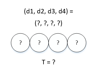
We begin by looking at the final position in the sequence. The completion date for the final job in the sequence is always known, since it is the summation of all job durations that need to be completed. In this example we know the final task will complete on day 24, as seen in table 2 above. Next we can calculate the delay that the final task will have, given it is the last job in the sequence, by subtracting the task due date from 24. After determining which job will yield the smallest delay when in the last position, we branch from that job and repeat the process for the second to last job in the sequence. Job A is due on day 5: 24 - 5 = 19 delay. Job B is due on day 6: 24 - 6 = 18 delay. Job C is due on day 16: 24 - 16 = 8 delay. Job D is due on day 14: 24 - 14 = 10 delay.
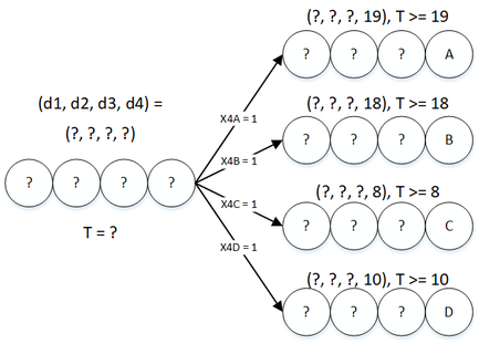
Figure 3 shows that job C in the final position of the sequence yields the smallest possible project delay T >= 8. Therefore, we branch from this path and repeat the process for the task in the second to last position. Since job C is selected to be last, and has a duration of 9 days, we know that the second to last job will be completed on day 15. From there we can once again use the known due dates of each task to determine the path with the smallest accrued delay. Job A is due on day 5: 15 - 5 = 10 delay. Job B is due on day 6: 15 - 6 = 9 delay. Job D is due on day 14: 15 - 14 = 1 delay.
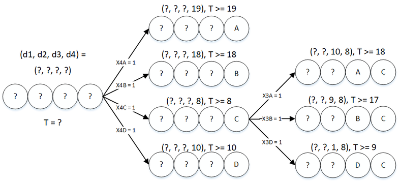
By continuing to determine the lower bound at each decision level, we eventually are left with only one option left for a job to take the first position. At this point we have determined our optimal solution, or the sequence yielding the smallest possible schedule delay. Figure 5 shows the completed Branch and Bound diagram, showing how an optimal solution of sequence: ABDC and a total project delay of T = 11 days can be achieved.

Applications
There are several ways in which the job-shop scheduling problem can be adapted, often to simplify the problem at hand, for a variety of applications. However, there are many distinctions that can be made between every utilization of the JSSP so there is continuous research ongoing to improve adaptability of the problem. Job-shop scheduling helps organizations to save valuable time and money
The most obvious example can be found in the manufacturing industry, as the name suggests. It is common for some production jobs to require certain machines to perform tasks, due to the proper capabilities or equipment of a given machine. This adds an additional layer to the problem, because not any job can be processed on any machine. This is known as flexible manufacturing. Furthermore, there are many uncertain factors that are not accounted for in the basic understanding of the problem, such as delays in delivery of necessary supplies, significant absence of workers, equipment malfunction, etc. [18]
This problem can also be applied to many projects in the technology industry. In computer programming, it is typical that computer instructions can only be executed one at a time on a single processor, sequentially. In this example of multiprocessor task scheduling, the instructions can be thought of as the "jobs" to be performed and the processors required for each task can be compared to the "machines". Here we would want to schedule the order of instructions such that the number of operations performed is maximized to make the computer as efficient as possible.[19]
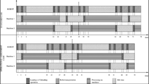
With the progression of automation in recent years, robotic tasks such as moving objects from one location to another are similarly optimized. In this application, the extent of movement of the robot is minimized while conducting the most amount of transport jobs to support the most effective productivity of the robot. There are additional nuances within this problem as well, such as the rotational movement capabilities of the robot, the layout of the robots within the system, and the number of parts or units the robot is able to produce. While each of these factors contribute to the complexity of the job shop scheduling problem, they are all worth considering as more and more companies are proceeding in this direction to reduce labor costs and increase flexibility and safety of the enterprise.[20]
Conclusions
JSSPs are used to optimize the allocation of shared resources in order to reduce the time and cost needed in order to complete a set amount of tasks. JSSPs account for the number of resources available, the operations needed to complete a job or task, the required order of operations, the necessary resources needed for each operation, as well as the necessary time needed with a resource for each operation in order to create an optimal schedule to complete all jobs. While this problem is used predominately for machining purposes, as the name implies, it can be adapted to be used on a variety of other cases within and outside of manufacturing. Other applications for this problem include the optimization of a computer's processing power as it executes multiple programs and optimization of automated equipment or robots.
References
- ↑ Joaquim A.S. Gromicho, Jelke J. van Hoorn, Francisco Saldanha-da-Gama, Gerrit T. Timmer, Solving the job-shop scheduling problem optimally by dynamic programming, Computers & Operations Research, Volume 39, Issue 12, 2012, Pages 2968-2977, ISSN 0305-0548, https://doi.org/10.1016/j.cor.2012.02.024.
- ↑ 2.0 2.1 2.2 T. Yamada and R. Nakano. "Job Shop Scheduling," IEEE Control Engineering Series, 1997.
- ↑ 3.0 3.1 A.S. Jain, S. Meeran, Deterministic job-shop scheduling: Past, present and future, European Journal of Operational Research, Volume 113, Issue 2, 1999, Pages 390-434, ISSN 0377-2217, https://www.sciencedirect.com/science/article/pii/S0377221798001131.
- ↑ P. Brucker, B. Jurisch and B. Sievers. "A branch and bound algorithm for the job-shop scheduling problem", Discrete Applied Mathematics, 1994.
- ↑ Abdeyazdan M., Rahmani A.M. (2008) Multiprocessor Task Scheduling using a new Prioritizing Genetic Algorithm based on number of Task Children. In: Kacsuk P., Lovas R., Németh Z. (eds) Distributed and Parallel Systems. Springer, Boston, MA. https://doi.org/10.1007/978-0-387-79448-8_10
- ↑ D. Applegate and W. Cook. "A computational study of the job-shop scheduling problem," ORSA J. on Comput, 1991.
- ↑ K. Hasan. "Evolutionary Algorithms for Solving Job-Shop Scheduling Problems in the Presence of Process Interruptions," Rajshahi University of Engineering and Technology, Bangladesh. 2009.
- ↑ Mohan, J., Lanka, K., & Rao, A. N. (2019). A Review of Dynamic Job Shop Scheduling Techniques, 30(Digital Manufacturing Transforming Industry Towards Sustainable Growth), 34–39. Retrieved from https://www.sciencedirect.com/science/article/pii/S2351978919300368
- ↑ Garey, M. R., Johnson, D. S. and Sethi, R. (1976) The Complexity of Flow Shop and Job-Shop Scheduling, Mathematics of Operations Research, May, 1(2), 117-129. https://www.jstor.org/stable/3689278
- ↑ Emmons, H., & Vairaktarakis, G. (2012). Flow Shop Scheduling: Theoretical . Springer New York Heidelberg Dordrecht London: Springer. https://books.google.com/books?hl=en&lr=&id=4UWMlwrescgC&oi=fnd&pg=PR3&dq=flow+shop+scheduling&ots=xz5Rkg6ATJ&sig=qSGDuAAjEmvhJosC9qng_1pZIA8#v=onepage&q=flow%20shop%20scheduling&f=false
- ↑ Sheldon B. Akers, Jr., (1956) Letter to the Editor—A Graphical Approach to Production Scheduling Problems. Operations Research 4(2):244-245. https://doi.org/10.1287/opre.4.2.244
- ↑ Coffman, E.G., Graham, R.L. Optimal scheduling for two-processor systems. Acta Informatica 1, 200–213 (1972). https://doi.org/10.1007/BF00288685
- ↑ N. Agin, Optimum seeking with branch and bound. Management Science, 13, 176-185, 1966. https://www.semanticscholar.org/paper/Optimum-Seeking-with-Branch-and-Bound-Agin/8d999d24c43d42685726a5658e3c279530e5b88f
- ↑ Jones, A., Rabelo, L. C., & Sharawi, A. T. (1999). Survey of job shop scheduling techniques. Wiley Encyclopedia of Electrical and Electronics Engineering. https://doi.org/10.1002/047134608x.w3352
- ↑ David Applegate, William Cook, (1991) A Computational Study of the Job-Shop Scheduling Problem. ORSA Journal on Computing 3(2):149-156. https://doi.org/10.1287/ijoc.3.2.149
- ↑ Morshed, M.S., Meeran, S., & Jain, A.S. (2017). A State-of-the-art Review of Job-Shop Scheduling Techniques. International Journal of Applied Operational Research - An Open Access Journal, 7, 0-0. https://neuro.bstu.by/ai/To-dom/My_research/Papers-0/For-courses/Job-SSP/jain.pdf
- ↑ https://www.youtube.com/watch?v=UGvc-qujB-o&ab_channel=YongWang
- ↑ Jianzhong Xu, Song Zhang, Yuzhen Hu, "Research on Construction and Application for the Model of Multistage Job Shop Scheduling Problem", Mathematical Problems in Engineering, vol. 2020, Article ID 6357394, 12 pages, 2020. https://doi.org/10.1155/2020/6357394
- ↑ Peter Brucker, "The Job-Shop Problem: Old and New Challenges", Universit¨at Osnabr¨uck, Albrechtstr. 28a, 49069 Osnabr¨uck, Germany, pbrucker@uni-osnabrueck.de
- ↑ 20.0 20.1 M.Selim Akturk, Hakan Gultekin, Oya Ekin Karasan, Robotic cell scheduling with operational flexibility, Discrete Applied Mathematics, Volume 145, Issue 3, 2005, Pages 334-348, ISSN 0166-218X