Derivative free optimization

Author: Brian Holcomb (bh597), Alejandra C Ramirez (mac593), Brian Worts (blw87), Trenton Berardi (tnb38), Ifeloluwa Osilaja (io62) (ChemE 6800 Fall 2024)

Stewards: Nathan Preuss, Wei-Han Chen, Tianqi Xiao, Guoqing Hu

Introduction

Derivative-Free Optimization (DFO) is a collection of computational methods used to find optimal values in situations where traditional optimization techniques that rely on derivatives are impractical or impossible to apply. Instead of requiring derivatives of an objective function, DFO methods iteratively search through a set of evaluated points to approximate an optimal solution. This approach is especially useful for black-box models where derivatives are unavailable, noisy, or computationally expensive to compute, such as in simulations, machine learning applications, or physical system modeling.

The motivation behind DFO emerged from a need to solve complex optimization problems in fields like engineering, finance, and logistics, where objective functions are often opaque or inaccessible for differentiation. Since the early 20th century, methods like pattern search and genetic algorithms have evolved, providing researchers with tools to tackle optimization in high-dimensional, uncertain environments. The primary goal of studying DFO is to enable efficient optimization when traditional methods fall short, particularly for models that are too complex or costly for gradient-based methods. DFO techniques have proven essential in areas like supply chain planning, engineering design, and financial modeling, where optimization can significantly impact operational efficiency and decision-making.

Algorithm Description

There are multiple methods of Derivative Free Optimization that are available. While DFO algorithms do not require you to calculate the derivative of the objective function, they rely on the algorithm to narrow the examined range of the objective function over multiple iterations by selecting points along the objective function and determining if the local minimum exists between these points. Two of these methods include Golden Section Search and Successive Parabolic Interpolation. Both operate in a similar fashion by evaluating the relationship between three points selected along the objective function and making decisions in order to narrow the examination window along the objective function where the points are selected for the next iteration. The main difference is how these three points are selected and how they are evaluated.

Golden Section Search

Golden Section Search gets its name from the ratio of points selected along the objective function which aligns closely to the Golden Ratio.

1. Identify a function, f(x), which you would like to find the minimum.

2. Select two points that are on both sides of the function’s minimum. Point a will be on the left side of the minimum and point b will be on the right side of the minimum. The section of function, f(x), between points a and b will form the examination window.

3. Select two more points called 𝑥1 and 𝑥2 as per the equation below. These will be spaced within the examination window from points a and b by the golden ratio as defined via constant c.

• 𝑥1 = 𝑐 ∗ 𝑎 + (1 - 𝑐) ∗ 𝑏
• 𝑥2 = (1 - 𝑐) ∗ 𝑎 + 𝑐 ∗ 𝑏
• 𝑐 = (―1 + 5)2

4. Evaluate and compare the objective function at 𝑥1 and 𝑥2 .

• If 𝑓(𝑥1) <= 𝑓(𝑥2) Then
  • Restrict the range of 𝑥 ∈ [𝑎,𝑥2].
  • 𝑏 = 𝑥2
  • 𝑥2 = 𝑥1
  • 𝑓2 = 𝑓1
  • 𝑥1 = 𝑐 ∗ 𝑎 + (1 - 𝑐) ∗ 𝑏
  • 𝑓1 = 𝑓(𝑥1)
• b. If 𝑓(𝑥1) > 𝑓(𝑥2) Then
  • Restrict the range of 𝑥 ∈ [𝑥1,𝑏].
  • 𝑎 = 𝑥1
  • 𝑥1 = 𝑥2
  • 𝑓1 = 𝑓2
  • 𝑥2 = (1 - 𝑐) ∗ 𝑎 + 𝑐 ∗ 𝑏
  • 𝑓2 = 𝑓(𝑥2)

5. After restricting the range as above recreate the variables 𝑎,𝑏,𝑥1,𝑥2 , based on similar structure as before, but with a narrowed range.

6. Iterate the function for n iteration loops or until the difference between variables a and b is a small number such as 1E-4.

Four images have been generated to describe the Golden Section Search Algorithm through 3 iterations.

Iteration 0

* Iteration 1

Iteration 2

Iteration 3

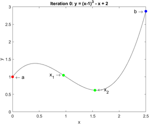
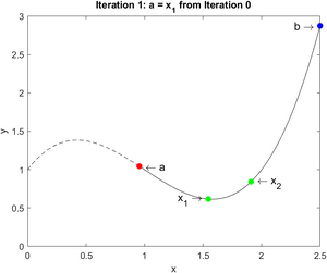
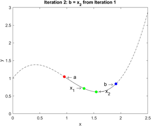
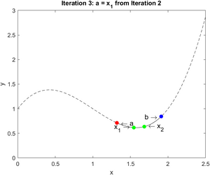
Successive Parabolic Interpolation

This algorithm leverages building a parabola defined by 3 points selected on a function f(x). The shape of the parabola is used to narrow the examined range on the function to

find where the function minimum is located. While the derivative of the objective function is not utilized, the derivative of the parabola is used.

1. Identify a function, f(x), that you wish to examine to find a minimum value.
2. Identify three points on the function, 𝑥1, 𝑥2, 𝑥3 . Two of the points will act as the outer bounds of the examination region and the third point will be in between these two.
3. Form a parabola between the three points identified on function f(x). The parabola can be defined using the Lagrange Interpolation Formula:
   • 𝑝(𝑥) = 𝑓(𝑥1) (𝑥 ― 𝑥2)(𝑥 ― 𝑥3) (𝑥1 ― 𝑥2)(𝑥1 ― 𝑥3) + 𝑓(𝑥2) (𝑥 ― 𝑥1)(𝑥 ― 𝑥3) (𝑥2 ― 𝑥1)(𝑥2 ― 𝑥3) + 𝑓(𝑥3) (𝑥 ― 𝑥1)(𝑥 ― 𝑥2) (𝑥3 ― 𝑥1)(𝑥3 ― 𝑥2)
4. The minimum of the parabola function will be where the first derivative of the parabola function equals to 0 and will align towards where the minimum of the function, 𝑓(𝑥), is located.
   • 𝑝′(𝑥0) = 0
   • 𝑥0 = 𝑥1 + 𝑥2 2 ― (𝑓(𝑥2) ― 𝑓(𝑥1))(𝑥3 ― 𝑥1)(𝑥3 ― 𝑥2) 2[(𝑥2 ― 𝑥1)(𝑓(𝑥3) ― 𝑓(𝑥2)) ― (𝑓(𝑥2) ― 𝑓(𝑥1))(𝑥3 ― 𝑥2)]
5. Compare the value of 𝑥0 to 𝑥2 and determine the next step for iteration.
   • If 𝑥0 <= 𝑥2 then shrink the examination range to be 𝑥 ∈ [𝑥1,𝑥2]
     • 𝑥𝑛𝑒𝑤1 = 𝑥𝑜𝑙𝑑1
     • 𝑥𝑛𝑒𝑤2= 𝑥0
     • 𝑥𝑛𝑒𝑤3 = 𝑥𝑜𝑙𝑑2
   • If 𝑥0 > 𝑥2 then shrink the examination range to be 𝑥 ∈ [𝑥2,𝑥3]
     • 𝑥𝑛𝑒𝑤1 = 𝑥𝑜𝑙𝑑2
     • 𝑥𝑛𝑒𝑤2 = 𝑥0
     • 𝑥𝑛𝑒𝑤3 = 𝑥𝑜𝑙𝑑3
6. Iterate the function for n iteration loops or until the difference between variables 𝑥1 and 𝑥3 is a small number such as 1E-4.

Numerical Examples

Example 1: Golden Section Search

Suppose we have a function 𝑓(𝑥) = (𝑥 - 2)2 +1, and we aim to find its minimum within the interval [𝑎,𝑏] = [0,5].

1. Initial Setup:

• Set 𝑎 = 0 and 𝑏 = 5
• Define the golden ratio constant 𝑐 ≈ 0.618
• Calculate two internal points within [𝑎,𝑏]
  • 𝑥1 = 𝑐 ∗ 𝑎 + (1 ― 𝑐) ∗ 𝑏 = 0.618 ∗ 0 + (1 ― 0.618) ∗ 5 ≈ 1.91
  • 𝑥2 = (1 ― 𝑐) ∗ 𝑎 + 𝑐 ∗ 𝑏 = (1 ― 0.618) ∗ 0 + 0.618 ∗ 5 ≈ 3.09

2. Iterative Evaluation:

• Evaluate 𝑓(𝑥1) = (1.91 ― 2)2 +1 ≈ and 𝑓(𝑥2) = (3.09 ― 2)2 +1 ≈ 2.19
• Since 𝑓(𝑥1) ≤ 𝑓(𝑥2), update the interval to [𝑎,𝑥2] = [0,3.09] and set 𝑏 = 𝑥2 = 3.09
• Recalculate:
  • New 𝑥2 = 𝑥1 ≈ 1.91
  • New 𝑥1 = 𝑐 ∗ 𝑎 +(1 ― 𝑐) ∗ 𝑏 ≈ 1.18

3. Convergence:

• Repeat this process, recalculating 𝑥1 and 𝑥2 and updating the interval until the difference between 𝑎 and 𝑏 is less than 10―4 .
• After a few iterations, the interval narrows around 𝑥 = 2, the minimum of the function, where 𝑓(𝑥) = 1.
• Two images have been generated to describe this numerical example through first iteration described above.

Iteration 0

Iteration 1

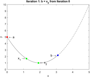
Example 2: Successive Parabolic Interpolation

Consider the same function 𝑓(𝑥) = (𝑥 ― 2)2 +1 and aim to find its minimum within an interval. Start with initial points 𝑥1 = 0, 𝑥2 = 2, and 𝑥3 = 4.

1. Initial Setup:

• Select points: 𝑥1 = 0, 𝑥2 = 2, and 𝑥3 = 4
• Evaluate 𝑓(𝑥1) = 5, 𝑓(𝑥2) = 1, and 𝑓(𝑥3) = 5

2. Parabolic Interpolation:

• Construct a parabola 𝑝(𝑥) through points (𝑥1, 𝑓(𝑥1)), (𝑥2, 𝑓(𝑥2)), and (𝑥3,𝑓(𝑥3)).
• Using the formula for 𝑥0 where 𝑝′(𝑥) = 0, calculate: 𝑥0 = 𝑥1 + 𝑥2 ― (𝑓(𝑥2) 𝑓(𝑥1))(𝑥3 𝑥1)(𝑥3 𝑥2) 2[(𝑥2 𝑥1)(𝑓(𝑥3) 𝑓(𝑥2)) (𝑓(𝑥2) 𝑓(𝑥1))(𝑥3 𝑥2)]
• Substituting values gives 𝑥0 ≈ 2, which is close to the minimum.

3. Updating the Interval:

• Since 𝑥0 ≈ 𝑥2 , shrink the interval to either [𝑥1,𝑥2] or [𝑥2,𝑥3] as needed.
• Set new points: 𝑥1 = 1, 𝑥2 = 𝑥0 ≈ 2,𝑥3 = 3.

4. Convergence:

• Repeat the iteration, adjusting points and recalculating 𝑥0 until the difference between 𝑥1 and 𝑥3 is less than 10―4 .
• The result converges around 𝑥 = 2, where the function minimum 𝑓(𝑥) = 1 is located.

Application

Oil and Gas

Derivative Free Optimization has a number of real world applications, including in the oil industry since often the cost functions and constraints require simulations of fluid mechanics where the gradient information cannot be obtained efficiently. This is an important problem that needs to be solved since oil and natural gas are the majority source of the current world’s energy supply so maximizing efficiency has global implications to the global economy and environments. Specifically, Derivative Free Optimization can be used, among other techniques, to optimize the production of oil. This is done by creating discretized simulations of very complex oil-water systems, using as many known variables as possible like fluid mechanics and seismic effects (Ciaurri, 2011). Thus, the minimization problem and its constraints become known and a search of the gradients becomes possible. Two such derivative-free optimization methods are the generalized pattern search and the Hookes-Jeeves Direct Search (Hooke, 1961). The generalized pattern search is a search algorithm for “derivative-free unconstrained optimization” divided into “search” and “poll” phases (Audet, 2000). In the search phase, a finite number of points are evaluated to find a minimum on a mesh. The poll phase is then used to poll the neighboring points on the mesh to find a better minimum before the process is repeated using a more refined mesh or an iterated search. The Hookes-Jeeves Direct Search method is a “Compass-based pattern search method” with an exploratory mode and a pattern mode, similar to that of the generalized pattern search (Hooke, 1961). In the exploratory mode, the local area is searched to refine the optima estimate while the pattern phase is used to identify patterns in the exploratory phase moves, which results in a better guess in the direction of the optima. Using these search methods to analyze their analysis results, the optimal control scheme to optimize oil production was determined. This was done by simulating using constraints for the water quantity, water to oil ratio, and resulting oil output while they searched for the optimal water pressure to use that minimizes cost (Ciaurri, 2011). They varied the configurations as well as utilized variations of the generalized pattern search and the Hookes-Jeeves Direct Search to search their gradients and find the optima. This work resulted in finding a feasible and optimal configuration scheme, expected profits, an increase in oil production, a decrease in water consumption, and thus showed how derivative-free computational optimization techniques can be applied to improve industries.

Engineering

Another real-world application of Derivative Free Optimization is for the minimization of the number of dampers to use to reduce the damage that tall buildings cause to each other during an earthquake in dense urban environments. Such events can put thousands of lives in danger and have caused billions of dollars in damage. Dampers are used to join adjacent buildings together to reduce the chance that they collide and increase the structural stability overall, but the upfront cost is extremely high so it is desirable to minimize the number of dampers that are required to put the building’s risk of damage in an earthquake within acceptable limits. Derivative Free Optimization, and specifically Model-Based Derivative Free Optimization, is the optimal choice for solving this kind of problem since the objective function is a “numerical integration” generated through an earthquake simulator that results in the optimizer not having access to the objective function gradients (Audet, 2017).

Medical

Using Model-Based Derivative Free Optimization consistently beats other methods in its efficiency of earthquake retrofitting optimization like Genetic Algorithms and Nelder-Mead since, in this application, the objective function appears to be differentiable which makes it an ideal use case (Audet, 2017). One application that highly relies on derivative-free optimization is the medical experimentation field. In the medical experimentation field derivative free optimization is often needed due to the complexity, noisy, non-differentiable functions or lack of ability to acquire data to obtain functions. An example of this is in cancer treatment where chemotherapy regimens involve 20+ independent variables with vast amounts of interdependent biological responses. Many biological responses are non-linear. Collection of testing combinations of these chemotherapy, dosage amounts, and interval timing between doses are not feasible; therefore there is not an ability to create a response function in order to use gradient optimization. Nelder and Mead (1964) and Box (1964) methods are example derivative-free optimization algorithms that have been used in this chemotherapy optimization problem. These are examples of Direct Search Methods (DSM) that help narrow the field of combinations of variables. A case study of this can be found in Berenbaum MC. “Direct search methods in the optimisation of cancer chemotherapy regimens (1990).” Nealder-Mead is a common optimizer option in common tools such as Excel, Python (Scipy) and Matlab.

Conclusion

Thanks to its robustness, Derivative-Free Optimization has emerged as a useful method of solving complex optimization problems where traditional methods that require derivatives to be available are not practical. This method of optimization is limited by the high computation cost, sensitivity to noise that leads to imperfect results, and the lack of gradient information that leads to slower convergence. However, advancements in computational power and algorithmic design are helping to mitigate these challenges, making DFO methods more efficient and accessible. There are numerous applications of Derivative-Free Optimization including in the oil, architecture, and medical industries where solving optimization problems has implications on global and local economies, the environment, and people’s health.

These examples demonstrate the usefulness that computational optimization has on humanity and its importance in our continuingly complex modern world. As the world continues to grow, environments continue to change, and better data becomes available, the methods of Derivative-Free Optimization will continue to grow with the world while helping humanity solve many of its most important challenges.

References

- ↑ 1.0 1.1 Ciaurri, D.E., Mukerji, T., Durlofsky, L.J. (2011). Derivative-Free Optimization for Oil Field Operations. In: Yang, XS., Koziel, S. (eds) Computational Optimization and Applications in Engineering and Industry. Studies in Computational Intelligence, vol 359. Springer, Berlin, Heidelberg. https://doi.org/10.1007/978-3-642-20986-4_2
- ↑ 2.0 2.1 Hooke, R., Jeeves, T.A.: Direct search solution of numerical and statistical problems. Journal of the ACM 8(2), 212–229 (1961)
- ↑ Audet, Charles & Dennis, J.. (2000). Analysis of Generalized Pattern Searches. SIAM Journal on Optimization. 13. 10.1137/S1052623400378742.
- ↑ 4.0 4.1 Audet, C., & Hare, W. (2017). Derivative-Free and Blackbox Optimization. Springer.
- ↑ Berenbaum MC. Direct search methods in the optimisation of cancer chemotherapy regimens. Br J Cancer. 1990 Jan;61(1):101-9. doi: 10.1038/bjc.1990.22. Erratum in: Br J Cancer 1990 May;61(5):788. PMID: 2297481; PMCID: PMC1971319. https://pmc.ncbi.nlm.nih.gov/articles/PMC1971319/