Simulated annealing: Difference between revisions
No edit summary |
|||
| Line 85: | Line 85: | ||
== Application == | == Application == | ||
SA is applied across diverse fields due to its effectiveness in solving complex optimization tasks, including areas like physics, engineering, data science, and finance. Some detailed examples are listed below. | SA is applied across diverse fields due to its effectiveness in solving complex optimization tasks, including areas like physics, engineering, data science, and finance. Some detailed examples are listed below. | ||
'''Job Scheduling in Manufacturing''' | |||
In job scheduling, the goal is to minimize the total production time (makespan) by optimally assigning tasks to machines. Traditional scheduling algorithms often get trapped in local minima due to the problem’s complexity. SA addresses this by allowing suboptimal solutions during the search process to escape local optima, eventually converging on a near-optimal schedule as the temperature decreases. | |||
Given an initial solution '''''x_current''''' representing a job sequence, the objective is to minimize the makespan: | |||
'''<math> min f(x) = makespan</math>''' | |||
where '''''f(x)''''' is the total completion time. SA perturbs the current sequence '''''x_current''''' to explore new solutions '''''x_new''''' and controls acceptance of suboptimal solutions by: | |||
<math>P = \exp (-\Delta E / T) </math> | |||
where '''''ΔE = f(x_new) - f(x_current)''''' and T is the temperature. A cooling schedule reduces '''''T''''' over iterations, focusing the search on refining the best solutions. | |||
'''Hyperparameter Tuning in Machine Learning''' | |||
Hyperparameter tuning is crucial for optimizing machine learning models. With SA, different combinations of hyperparameters are treated as solutions, and the algorithm explores this space to find the best configuration. By allowing suboptimal combinations early on, SA avoids getting stuck in poor configurations, converging on an optimal setting as it cools. | |||
'''Path Optimization in Robotics''' | |||
SA is widely used in robotics for path optimization, where the goal is to find the shortest or most efficient path for a robot to follow. The algorithm treats each path configuration as a solution and iteratively refines it by accepting suboptimal paths temporarily. As temperature decreases, SA converges to an optimal or near-optimal path, balancing exploration and refinement. | |||
'''Inventory Optimization in Supply Chain''' | |||
SA is also applied in inventory management to find an optimal stock level that balances storage costs and service levels. Starting with an initial inventory policy, SA perturbs the policy to explore new configurations and accepts costlier policies initially to escape local optima. Over time, the solution converges to a cost-effective policy. | |||
'''Other Applications''' | |||
SA has applications in diverse areas like finance (portfolio optimization), logistics (route optimization), and artificial intelligence (feature selection). For example, in portfolio optimization, SA can optimize asset weights to balance risk and return, allowing for high-risk portfolios initially before settling on a balanced configuration. | |||
== Conclusion == | == Conclusion == | ||
SA since its introduction in the 1980s, has been widely adopted as an effective optimization technique due to its ability to escape local minima and handle complex search spaces. Its probabilistic approach based on metallurgical annealing processes makes it particularly suitable for combinatorial optimization problems where deterministic methods struggle. SA has found successful applications across diverse fields including manufacturing job scheduling, machine learning hyperparameter tuning, robotics path planning, supply chain optimization, and financial portfolio management, demonstrating its versatility and practical value in solving real-world optimization challenges. | SA since its introduction in the 1980s, has been widely adopted as an effective optimization technique due to its ability to escape local minima and handle complex search spaces. Its probabilistic approach based on metallurgical annealing processes makes it particularly suitable for combinatorial optimization problems where deterministic methods struggle. SA has found successful applications across diverse fields including manufacturing job scheduling, machine learning hyperparameter tuning, robotics path planning, supply chain optimization, and financial portfolio management, demonstrating its versatility and practical value in solving real-world optimization challenges. | ||
Revision as of 01:47, 14 December 2024
Author: Gwen Zhang (xz929), Yingjie Wang (yw2749), Junchi Xiao (jx422), Yichen Li (yl3938), Xiaoxiao Ge (xg353) (ChemE 6800 Fall 2024)
Stewards: Nathan Preuss, Wei-Han Chen, Tianqi Xiao, Guoqing Hu
Introduction
Simulated annealing (SA) is a probabilistic optimization algorithm inspired by the metallurgical annealing process, which reduces defects in a material by controlling the cooling rate to achieve a stable state.[1] The core concept of SA is to allow algorithms to escape the constraints of local optima by occasionally accepting suboptimal solutions. This characteristic enables SA to find near-global optima in large and complex search spaces.[2] During the convergence process, the probability of accepting a suboptimal solution diminishes over time.
SA is widely applied in diverse fields such as scheduling,[3] machine learning, and engineering design, and is particularly effective for combinatorial optimization problems that are challenging for deterministic methods.[4] First proposed in the 1980s by Kirkpatrick, Gelatt, and Vecchi, SA demonstrated its efficacy in solving various complex optimization problems through its analogy to thermodynamics.[5] Today, it remains a powerful heuristic often combined with other optimization techniques to enhance performance in challenging problem spaces.
Algorithm Discussion
Formal Description of the Algorithm
SA is a probabilistic technique for finding approximate solutions to optimization problems, particularly those with large search spaces. Inspired by the annealing process in metallurgy, the algorithm explores the solution space by occasionally accepting worse solutions with a probability that diminishes over time. This reduces the risk of getting stuck in local optima and increases the likelihood of discovering the global optimum.
The basic steps of the SA algorithm are as follows:
- Initialization: Begin with an initial solution $ s_0 $ and an initial temperature $ T_0 $.
- Iterative Improvement: While the stopping criteria are not met:
- Generate a new solution $ s_{new} $ in the neighborhood of the current solution s.
- Calculate the difference in objective values $ \Delta E = f(s_{new}) - f(s) $, where $ f $ is the objective function.
- If $ \Delta E <0 $ (i.e., $ s_{new} $ is a better solution), accept $ s_{new} $ as the current solution.
- If $ \Delta E >0 $, accept $ s_{new} $ with a probability $ P = \exp\left(-\frac{\Delta E}{T}\right) $.
- Update the temperature $ T $ according to a cooling schedule, typically $ T=\alpha \cdot T $, where $ \alpha $ is a constant between 0 and 1.
- Termination: Stop the process when the temperature falls below a minimum threshold , or after a predefined number of iterations. The best solution encountered is returned as the approximate optimum.
Pseudocode for Simulated Annealing
def SimulatedAnnealing(f, s_0, T_0, alpha, T_min):
    s_current = s_0
    T = T_0
    while T > T_min:
        s_new = GenerateNeighbor(s_current)
        delta_E = f(s_new) - f(s_current)
        if delta_E < 0 or Random(0, 1) < math.exp(-delta_E / T):
            s_current = s_new
        T = alpha * T
    return s_current
Assumptions and Conditions
Objective Function Continuity
The objective function $ f $ is assumed to be defined and continuous in the search space.
Cooling Schedule
The cooling schedule, typically geometric, determines how $ T $ decreases over iterations. The cooling rate $ \alpha $ affects the convergence speed and solution quality.
Acceptance Probability
Based on the Metropolis criterion, the probability $ P = \exp\left(-\frac{\Delta E}{T}\right) $ allows the algorithm to accept worse solutions initially, encouraging broader exploration.
Termination Condition
SA terminates when $ T $ falls below $ T_{min} $ or when a predefined number of iterations is reached.
Numerical Examples

The Ising model is a classic example from statistical physics and in order to reach its optimal state, we can use Simulated Annealing (SA) to reach a minimal energy state.[6] In the SA approach, we start with a high "temperature" that allows random changes in the system’s configuration, which helps explore different arrangements of spins. As the temperature lowers, the algorithm gradually favors configurations with lower energy, eventually "freezing" into a low-energy state.
Problem Setup
Consider a small $ 2\times 2 $ grid of spins, where each spin can be either $ +1 $ or $ -1 $ . The energy of the system is determined by the Hamiltonian: $ E = -J \sum_{\langle i,j \rangle} S_i S_j $, where $ J $ is a coupling constant (set to 1 for simplicity), $ s_i $ and $ s_j $ are neighboring spins, and the summation is over nearest neighbors. The goal is to minimize $ E $, achieved when all spins are aligned.
Algorithm Steps
- Initialize the spins: start with a random configuration. For example: $ L = \begin{bmatrix} +1 & -1 \\ -1 & +1 \end{bmatrix} $
- Calculate Initial Energy: For this configuration, each pair of neighboring spins contributes $ -JS_i S_j $ to the energy. Calculate by summing these contributions: The pairs are $ (+1, -1), (-1, +1), (-1, +1), (+1, -1) $, all of which contribute $ +1 $. So, initial energy $ E = 4 $.
- Neighboring Configurations: Select a random spin to flip. Suppose the spin in the top right corner is chosen, changing $ +1 $ to $ -1 $: $ \text{New L} = \begin{bmatrix} +1 & +1 \\ -1 & +1 \end{bmatrix} $ Recalculate $ E $ for the new configuration: Now, three pairs are aligned $ (+1,+1) $ and contribute $ -1 $ each, while one pair $ (-1,+1) $ contributes $ +1 $, so total energy $ E = -2 $.
- Acceptance Decision: Calculate $ \Delta E = E_{\text{new}} - E_{\text{old}} = -2 - 4 = -6 $. Since $ \Delta E < 0 $, accept the new configuration.
- Cooling Schedule: Reduce the temperature $ T $ gradually to decrease the likelihood of accepting higher-energy configurations.
- Iterate: Continue flipping spins randomly, recalculating energy, and applying the acceptance criterion until the system reaches a low-energy configuration (e.g., all $ +1 $ or all $ -1 $). After several iterations at decreasing temperatures, the system is likely to converge to a minimum-energy configuration, such as: $ \begin{bmatrix} +1 & +1 \\ +1 & +1 \end{bmatrix} \quad \text{or} \quad \begin{bmatrix} -1 & -1 \\ -1 & -1 \end{bmatrix} $as shown.
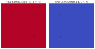
Figure 2: Two Final configurations

Application
SA is applied across diverse fields due to its effectiveness in solving complex optimization tasks, including areas like physics, engineering, data science, and finance. Some detailed examples are listed below.
Job Scheduling in Manufacturing
In job scheduling, the goal is to minimize the total production time (makespan) by optimally assigning tasks to machines. Traditional scheduling algorithms often get trapped in local minima due to the problem’s complexity. SA addresses this by allowing suboptimal solutions during the search process to escape local optima, eventually converging on a near-optimal schedule as the temperature decreases.
Given an initial solution x_current representing a job sequence, the objective is to minimize the makespan:
$ min f(x) = makespan $
where f(x) is the total completion time. SA perturbs the current sequence x_current to explore new solutions x_new and controls acceptance of suboptimal solutions by:
$ P = \exp (-\Delta E / T) $
where ΔE = f(x_new) - f(x_current) and T is the temperature. A cooling schedule reduces T over iterations, focusing the search on refining the best solutions.
Hyperparameter Tuning in Machine Learning
Hyperparameter tuning is crucial for optimizing machine learning models. With SA, different combinations of hyperparameters are treated as solutions, and the algorithm explores this space to find the best configuration. By allowing suboptimal combinations early on, SA avoids getting stuck in poor configurations, converging on an optimal setting as it cools.
Path Optimization in Robotics
SA is widely used in robotics for path optimization, where the goal is to find the shortest or most efficient path for a robot to follow. The algorithm treats each path configuration as a solution and iteratively refines it by accepting suboptimal paths temporarily. As temperature decreases, SA converges to an optimal or near-optimal path, balancing exploration and refinement.
Inventory Optimization in Supply Chain
SA is also applied in inventory management to find an optimal stock level that balances storage costs and service levels. Starting with an initial inventory policy, SA perturbs the policy to explore new configurations and accepts costlier policies initially to escape local optima. Over time, the solution converges to a cost-effective policy.
Other Applications
SA has applications in diverse areas like finance (portfolio optimization), logistics (route optimization), and artificial intelligence (feature selection). For example, in portfolio optimization, SA can optimize asset weights to balance risk and return, allowing for high-risk portfolios initially before settling on a balanced configuration.
Conclusion
SA since its introduction in the 1980s, has been widely adopted as an effective optimization technique due to its ability to escape local minima and handle complex search spaces. Its probabilistic approach based on metallurgical annealing processes makes it particularly suitable for combinatorial optimization problems where deterministic methods struggle. SA has found successful applications across diverse fields including manufacturing job scheduling, machine learning hyperparameter tuning, robotics path planning, supply chain optimization, and financial portfolio management, demonstrating its versatility and practical value in solving real-world optimization challenges.
- ↑ Metropolis, N., Rosenbluth, A. W., Rosenbluth, M. N., Teller, A. H., & Teller, E.(1953). "Equation of state calculations by fast computing machines." Journal of Chemical Physics, 21(6), 1087-1092.
- ↑ Kirkpatrick, S., Gelatt, C. D., & Vecchi, M. P. (1983). "Optimization by simulated annealing." Science, 220(4598), 671-680.
- ↑ Aarts, E. H., & Korst, J. H. (1988). Simulated Annealing and Boltzmann Machines: A Stochastic Approach to Combinatorial Optimization and Neural Computing. Wiley.
- ↑ Cerny, V. (1985). "Thermodynamical approach to the traveling salesman problem: An efficient simulation algorithm." Journal of Optimization Theory and Applications, 45(1), 41-51.
- ↑ Kirkpatrick, S. (1984). "Optimization by simulated annealing: Quantitative studies." Journal of Statistical Physics, 34(5-6), 975-986.
- ↑ Peierls, R. (1936). On Ising’s model of ferromagnetism. Mathematical Proceedings of the Cambridge Philosophical Society, 32(3), 477–481.