Subgradient optimization: Difference between revisions
SYSEN5800TAs (talk | contribs) No edit summary |
Initial Changes (Introduction, Application, and Conclusion) |
||
| Line 4: | Line 4: | ||
[[File:Subderivative_illustration.png|right|thumb|A convex nondifferentiable function (blue) with red "subtangent" lines generalizing the derivative at the nondifferentiable point ''x''<sub>0</sub>.]] | [[File:Subderivative_illustration.png|right|thumb|A convex nondifferentiable function (blue) with red "subtangent" lines generalizing the derivative at the nondifferentiable point ''x''<sub>0</sub>.]] | ||
''' | The '''subgradient method''' is a simple algorithm for the optimization of non-differentiable functions, and it originated in the Soviet Union during the 1960s and 70s, primarily by the contributions of Naum Z. Shor (Sharma, Shashi). While the calculations for this approach are similar to that of the gradient method for differentiable functions, there are several key differences. First, as noted the subgradient method applies strictly to non-differentiable functions as it reduces to the gradient method when f is differentiable. Secondly the step size is fixed before the application of the algorithm rather than being determined “on-line” as in other approaches. Finally the subgradient method is not a descent method as the value of f can and often will increase. | ||
==Introduction== | ==Introduction== | ||
The ' | The subgradient method is more computationally expensive when compared to Newton's method but applicable to a wider range of problems. Additionally, due to the method’s schema when applied numerically the memory requirements are smaller than other methods allowing larger problems to be approached. Further the combination of the subgradient method with the primal dual decomposition can simplify some applications to a distributed algorithm. | ||
==Algorithm Discussion== | |||
Basics: | |||
Starting with a convex function f such that f:RnR with domain Rn. The classic implementation of the sub-gradient method iterates: | |||
x(k+1)=x(k)-kg(k) | |||
The subgradient method is more computationally expensive when compared to Newton's method but applicable to a wider range of problems. Additionally, due to the method’s schema when applied numerically the memory requirements are smaller than other methods allowing larger problems to be approached. Further the combination of the subgradient method with the primal dual decomposition can simplify some applications to a distributed algorithm. | |||
<math>g</math> is a subgradient of <math>f</math> at <math>x</math> if, for all <math>y</math>, the following is true: <br/> | |||
[[File:Subgradient.png|200px|center]] | [[File:Subgradient.png|200px|center]] | ||
An example of the subgradient of a nondifferentiable convex function <math>f</math> can be seen below: | An example of the subgradient of a nondifferentiable convex function <math>f</math> can be seen below: | ||
| Line 63: | Line 71: | ||
This figure illustrates that both the nonsummable diminishing step size rule and the square summable but not summable step size rule show relatively fast and good convergence. The square summable but not summable step size rule shows less variation than the nonsummable diminishing step size rule but both show similar speed and convergence. <br/> | This figure illustrates that both the nonsummable diminishing step size rule and the square summable but not summable step size rule show relatively fast and good convergence. The square summable but not summable step size rule shows less variation than the nonsummable diminishing step size rule but both show similar speed and convergence. <br/> | ||
Overall, all four step size rules can be used to get good convergence, so it is important to try different values for <math>h</math> in the constant step size and length rules and different formulas for the nonsummable diminishing step size rule and the square summable but not summable step size rule in order to get good convergence in the smallest amount of iterations possible. | Overall, all four step size rules can be used to get good convergence, so it is important to try different values for <math>h</math> in the constant step size and length rules and different formulas for the nonsummable diminishing step size rule and the square summable but not summable step size rule in order to get good convergence in the smallest amount of iterations possible. | ||
==Application== | |||
Subgradient methods are generally for solving non-differentiable optimization problems. This algorithm is used in data science applications such as machine learning whenever the gradient method is not sufficient. It is also found in applications like engineering where it is utilized for problems in robotics and power systems (Licio, Romao). | |||
In some applications, the combination of the subgradient method and the primal dual decomposition can simplify to a distributed algorithm. This is shown in detail in Adaptive Subgradient Methods for Online Learning and Stochastic Optimization (Duchi et al.). The experiments outlined focus on different data sets such as text and images, and then use the subgradient method in order to flexibly be applied in various geometries. This adaptive characteristic provides unique benefits such as improved performance for identification of predictive attributes when compared to non-adaptive alternatives. | |||
Some commercial tools like MATLAB and optimization solvers like Gurobi, FICO, and MOSEK contain the subgradient method algorithm. There are also open-source solvers like Couenee and GLPK that support this function. Alternatively, CVXPY is an open-source Python embedded modeling language that contains subgradient methods in its library. | |||
==Conclusion== | ==Conclusion== | ||
In summary, the subgradient method is a simple algorithm for the optimization of non-differentiable functions. While its performance is not as desirable as other algorithms, its simplicity and adaptability to problem formulation keeps it in use for a number of applications. As always, problem formulation should be a key consideration in the selection of this algorithm. A number of variations on step size and solutions exist extending the applicability of this method and it should be considered for the case of non-differentiable problems. | |||
==References== | ==References== | ||
Revision as of 20:48, 14 December 2024
Author: Malichi Merski (mm2835), Ryan Ortiz (rjo64), Nicholas Phillips (ntp28) (ChemE 6800 Fall 2024)
Stewards: Nathan Preuss, Wei-Han Chen, Tianqi Xiao, Guoqing Hu
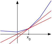
The subgradient method is a simple algorithm for the optimization of non-differentiable functions, and it originated in the Soviet Union during the 1960s and 70s, primarily by the contributions of Naum Z. Shor (Sharma, Shashi). While the calculations for this approach are similar to that of the gradient method for differentiable functions, there are several key differences. First, as noted the subgradient method applies strictly to non-differentiable functions as it reduces to the gradient method when f is differentiable. Secondly the step size is fixed before the application of the algorithm rather than being determined “on-line” as in other approaches. Finally the subgradient method is not a descent method as the value of f can and often will increase.
Introduction
The subgradient method is more computationally expensive when compared to Newton's method but applicable to a wider range of problems. Additionally, due to the method’s schema when applied numerically the memory requirements are smaller than other methods allowing larger problems to be approached. Further the combination of the subgradient method with the primal dual decomposition can simplify some applications to a distributed algorithm.
Algorithm Discussion
Basics: Starting with a convex function f such that f:RnR with domain Rn. The classic implementation of the sub-gradient method iterates: x(k+1)=x(k)-kg(k)
The subgradient method is more computationally expensive when compared to Newton's method but applicable to a wider range of problems. Additionally, due to the method’s schema when applied numerically the memory requirements are smaller than other methods allowing larger problems to be approached. Further the combination of the subgradient method with the primal dual decomposition can simplify some applications to a distributed algorithm.
$ g $ is a subgradient of $ f $ at $ x $ if, for all $ y $, the following is true:

An example of the subgradient of a nondifferentiable convex function $ f $ can be seen below:

Where $ g_1 $ is a subgradient at point $ x_1 $ and $ g_2 $ and $ g_3 $ are subgradients at point $ x_2 $. Notice that when the function is differentiable, such as at point $ x_1 $, the subgradient, $ g_1 $, just becomes the gradient to the function. Other important factors of the subgradient to note are that the subgradient gives a linear global underestimator of $ f $ and if $ f $ is convex, then there is at least one subgradient at every point in its domain. The set of all subgradients at a certain point is called the subdifferential, and is written as $ \partial f(x_0) $ at point $ x_0 $.
The Subgradient Method
Suppose $ f:\mathbb{R}^n \to \mathbb{R} $ is a convex function with domain $ \mathbb{R}^n $. To minimize $ f $ the subgradient method uses the iteration:

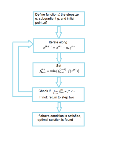
Where $ k $ is the number of iterations, $ x^{(k)} $ is the $ k $th iterate, $ g^{(x)} $ is any subgradient at $ x^{(k)} $, and $ \alpha_k $$ (> 0) $ is the $ k $th step size. Thus, at each iteration of the subgradient method, we take a step in the direction of a negative subgradient. As explained above, when $ f $ is differentiable, $ g^{(k)} $ simply reduces to $ \nabla $$ f(x^{(k)}) $. It is also important to note that the subgradient method is not a descent method in that the new iterate is not always the best iterate. Thus we need some way to keep track of the best solution found so far, i.e. the one with the smallest function value. We can do this by, after each step, setting

and setting $ i_{\text{best}}^{(k)} = k $ if $ x^{(k)} $ is the best (smallest) point found so far. Thus we have:

which gives the best objective value found in $ k $ iterations. Since this value is decreasing, it has a limit (which can be $ -\infty $).
An algorithm flowchart is provided below for the subgradient method:
Step size
Several different step size rules can be used:
- Constant step size: $ \alpha_k = h $ independent of $ k $.
- Constant step length:
 This means that
- Square summable but not summable: These step sizes satisfy
- Nonsummable diminishing: These step sizes satisfy
An important thing to note is that for all four of the rules given here, the step sizes are determined "off-line", or before the method is iterated. Thus the step sizes do not depend on preceding iterations. This "off-line" property of subgradient methods differs from the "on-line" step size rules used for descent methods for differentiable functions where the step sizes do depend on preceding iterations.
Convergence Results
There are different results on convergence for the subgradient method depending on the different step size rules applied. For constant step size rules and constant step length rules the subgradient method is guaranteed to converge within some range of the optimal value. Thus:

where $ f^{*} $ is the optimal solution to the problem and $ \epsilon $ is the aforementioned range of convergence. This means that the subgradient method finds a point within $ \epsilon $ of the optimal solution $ f^{*} $. $ \epsilon $ is number that is a function of the step size parameter $ h $, and as $ h $ decreases the range of convergence $ \epsilon $ also decreases, i.e. the solution of the subgradient method gets closer to $ f^{*} $ with a smaller step size parameter $ h $.
For the diminishing step size rule and the square summable but not summable rule, the algorithm is guaranteed to converge to the optimal value or ![]() When the function $ f $ is differentiable the subgradient method with constant step size yields convergence to the optimal value, provided the parameter $ h $ is small enough.
When the function $ f $ is differentiable the subgradient method with constant step size yields convergence to the optimal value, provided the parameter $ h $ is small enough.
Example: Piecewise linear minimization
Suppose we wanted to minimize the following piecewise linear convex function using the subgradient method:

Since this is a linear programming problem finding a subgradient is simple: given $ x $ we can find an index $ j $ for which:

The subgradient in this case is $ g=a_j $. Thus the iterative update is then:

Where $ j $ is chosen such to satisfy ![]() In order to apply the subgradient method to this problem all that is needed is some way to calculate
In order to apply the subgradient method to this problem all that is needed is some way to calculate ![]() and the ability to carry out the iterative update. Even if the problem is dense and very large (where standard linear programming might fail), if there is some efficient way to calculate $ f $ then the subgradient method is a reasonable choice for algorithm.
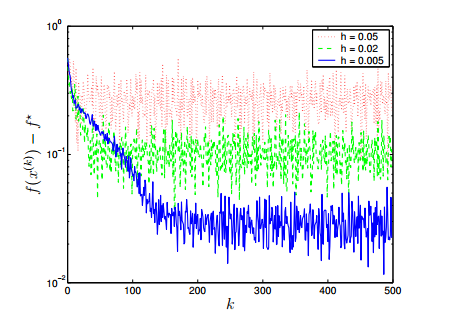
Consider a problem with $ n=10 $ variables and $ m=100 $ terms and with data $ a_i $ and $ b_i $ generated from a normal distribution. We will consider all four of the step size rules mentioned above and will plot $ \epsilon $ or the difference between the optimal solution and the subgradient solution as a function of $ k $, the nuber of iterations.
and the ability to carry out the iterative update. Even if the problem is dense and very large (where standard linear programming might fail), if there is some efficient way to calculate $ f $ then the subgradient method is a reasonable choice for algorithm.
Consider a problem with $ n=10 $ variables and $ m=100 $ terms and with data $ a_i $ and $ b_i $ generated from a normal distribution. We will consider all four of the step size rules mentioned above and will plot $ \epsilon $ or the difference between the optimal solution and the subgradient solution as a function of $ k $, the nuber of iterations.
For the constant step size rule ![]() for several values of $ h $ the following plot was obtained:
for several values of $ h $ the following plot was obtained:
For the constant step length rule ![]() for several values of $ h $ the following plot was obtained:
for several values of $ h $ the following plot was obtained:
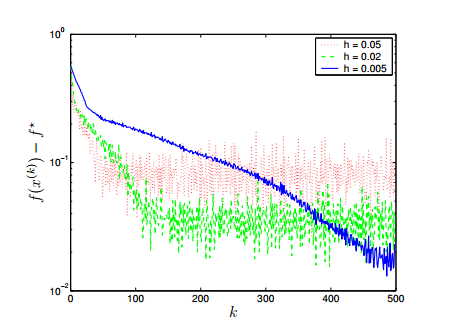
The above figures reveal a trade-off: a larger step size parameter $ h $ gives a faster convergence but in the end gives a larger range of suboptimality so it is important to determine an $ h $ that will converge close to the optimal solution without taking a very large number of iterations.
For the subgradient method using diminishing step size rules, both the nonsummable diminishing step size rule ![]() (blue) and the square summable but not summable step size rule
(blue) and the square summable but not summable step size rule ![]() (red) are plotted below for convergence:
(red) are plotted below for convergence:
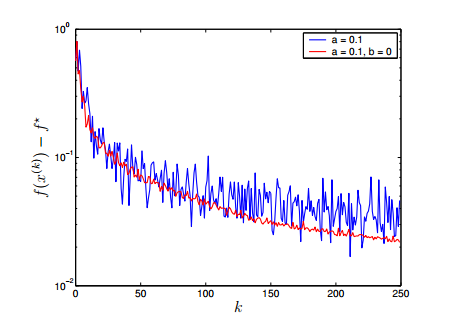
This figure illustrates that both the nonsummable diminishing step size rule and the square summable but not summable step size rule show relatively fast and good convergence. The square summable but not summable step size rule shows less variation than the nonsummable diminishing step size rule but both show similar speed and convergence.
Overall, all four step size rules can be used to get good convergence, so it is important to try different values for $ h $ in the constant step size and length rules and different formulas for the nonsummable diminishing step size rule and the square summable but not summable step size rule in order to get good convergence in the smallest amount of iterations possible.
Application
Subgradient methods are generally for solving non-differentiable optimization problems. This algorithm is used in data science applications such as machine learning whenever the gradient method is not sufficient. It is also found in applications like engineering where it is utilized for problems in robotics and power systems (Licio, Romao).
In some applications, the combination of the subgradient method and the primal dual decomposition can simplify to a distributed algorithm. This is shown in detail in Adaptive Subgradient Methods for Online Learning and Stochastic Optimization (Duchi et al.). The experiments outlined focus on different data sets such as text and images, and then use the subgradient method in order to flexibly be applied in various geometries. This adaptive characteristic provides unique benefits such as improved performance for identification of predictive attributes when compared to non-adaptive alternatives.
Some commercial tools like MATLAB and optimization solvers like Gurobi, FICO, and MOSEK contain the subgradient method algorithm. There are also open-source solvers like Couenee and GLPK that support this function. Alternatively, CVXPY is an open-source Python embedded modeling language that contains subgradient methods in its library.
Conclusion
In summary, the subgradient method is a simple algorithm for the optimization of non-differentiable functions. While its performance is not as desirable as other algorithms, its simplicity and adaptability to problem formulation keeps it in use for a number of applications. As always, problem formulation should be a key consideration in the selection of this algorithm. A number of variations on step size and solutions exist extending the applicability of this method and it should be considered for the case of non-differentiable problems.
References
1. Akgul, M. "Topics in Relaxation and Ellipsoidal Methods", volume 97 of Research Notes in Mathematics. Pitman, 1984.
2. Bazaraa, M. S., Sherali, H. D. "On the choice of step size in subgradient optimization." European Journal of Operational Research 7.4, 1981
3. Bertsekas, D. P. "Nonlinear Programming", (2nd edition), Athena Scientific, Belmont, MA, 1999.
4. Goffin, J. L. "On convergence rates of subgradient optimization methods." Mathematical Programming 13.1, 1977.
5. Shor, N. Z. "Minimization Methods for Non-differentiable Functions". Springer Series in Computational Mathematics. Springer, 1985.
6. Shor, N. Z. "Nondifferentiable Optimization and Polynomial Problems". Nonconvex Optimization and its Applications. Kluwer, 1998.