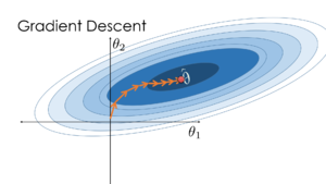
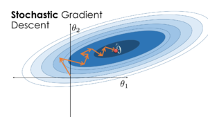
Stochastic gradient descent

Authors: Jonathon Price, Alfred Wong, Tiancheng Yuan, Joshua Mathews, Taiwo Olorunniwo (SYSEN 5800 Fall 2020)
Steward: Fengqi You

Introduction

Stochastic gradient descent (abbreviated as SGD) is an iterative method often used for machine learning, optimizing the gradient descent during each search once a random weight vector is picked. The gradient descent is a strategy that searches through a large or infinite hypothesis space whenever 1) there are hypotheses continuously being parameterized and 2) the errors are differentiable based on the parameters. The problem with gradient descent is that converging to a local minimum takes extensive time and determining a global minimum is not guaranteed. In SGD, the user initializes the weights and the process updates the weight vector using one data point. The gradient descent continuously updates it incrementally when an error calculation is completed to improve convergence. The method seeks to determine the steepest descent and it reduces the number of iterations and the time taken to search large quantities of data points. Over the recent years, the data sizes have increased immensely such that current processing capabilities are not enough. Stochastic gradient descent is being used in neural networks and decreases machine computation time while increasing complexity and performance for large-scale problems.

Theory

Visualization of the gradient descent algorithm

SGD is a variation on gradient descent, also called batch gradient descent. As a review, gradient descent seeks to minimize an objective function $J(\theta )$ by iteratively updating each parameter $\theta$ by a small amount based on the negative gradient of a given data set. The steps for performing gradient descent are as follows:

Step 1: Select a learning rate $\alpha$

Step 2: Select initial parameter values $\theta$ as the starting point

Step 3: Update all parameters from the gradient of the training data set, i.e. compute $\theta _{i+1}=\theta _{i}-\alpha \times {\nabla _{\theta }}J(\theta )$

Step 4: Repeat Step 3 until a local minima is reached

Under batch gradient descent, the gradient, ${\nabla _{\theta }}J(\theta )$, is calculated at every step against a full data set. When the training data is large, computation may be slow or require large amounts of computer memory.

Visualization of the stochastic gradient descent algorithm

Stochastic Gradient Descent Algorithm

SGD modifies the batch gradient descent algorithm by calculating the gradient for only one training example at every iteration. The steps for performing SGD are as follows:

Step 1: Randomly shuffle the data set of size m

Step 2: Select a learning rate $\alpha$

Step 3: Select initial parameter values $\theta$ as the starting point

Step 4: Update all parameters from the gradient of a single training example $x^{j},y^{j}$, i.e. compute $\theta _{i+1}=\theta _{i}-\alpha \times {\nabla _{\theta }}J(\theta ;x^{j};y^{j})$

Step 5: Repeat Step 4 until a local minimum is reached

By calculating the gradient for one data set per iteration, SGD takes a less direct route towards the local minimum. However, SGD has the advantage of having the ability to incrementally update an objective function $J(\theta )$ when new training data is available at minimum cost.

Learning Rate

The learning rate is used to calculate the step size at every iteration. Too large a learning rate and the step sizes may overstep too far past the optimum value. Too small a learning rate may require many iterations to reach a local minimum. A good starting point for the learning rate is 0.1 and adjust as necessary.

Mini-Batch Gradient Descent

A variation on stochastic gradient descent is the mini-batch gradient descent. In SGD, the gradient is computed on only one training example and may result in a large number of iterations required to converge on a local minimum. Mini-batch gradient descent offers a compromise between batch gradient descent and SGD by splitting the training data into smaller batches. The steps for performing mini-batch gradient descent are identical to SGD with one exception - when updating the parameters from the gradient, rather than calculating the gradient of a single training example, the gradient is calculated against a batch size of $n$ training examples, i.e. compute $\theta _{i+1}=\theta _{i}-\alpha \times {\nabla _{\theta }}J(\theta ;x^{j:j+n};y^{j:j+n})$

Numerical Example

Data preparation

Consider a simple 2-D data set with only 6 data points (each point has $x_{1},x_{2}$), and each data point have a label value $y$ assigned to them.

Model overview

For the purpose of demonstrating the computation of the SGD process, simply employ a linear regression model: $y=w_{1}\ x_{1}+w_{2}\ x_{2}+b$, where $w_{1}$ and $w_{2}$ are weights and $b$ is the constant term. In this case, the goal of this model is to find the best value for $w_{1},w_{2}$ and $b$, based on the datasets.

Definition of loss function

In this example, the loss function should be l2 norm square, that is $L=({\widehat {y}}-y)^{2}$.

Forward

Initial Weights:

The linear regression model starts by initializing the weights $w_{1},w_{2}$ and setting the bias term at 0. In this case, initiate [$w_{1},w_{2}$] = [-0.044, -0.042].

Dataset:

In this problem, we set 1 as the batch size. And the entire dataset of [ $x_{1}$, $x_{2}$, $y$] is given by:

Caption text

$x_{1}$	$x_{2}$	$y$
4	1	2
2	8	-14
1	0	1
3	2	-1
1	4	-7
6	7	-8

Gradient Computation and Parameter Update

The purpose of BP is to obtain the impact of the weights and bias terms for the entire model.  The update of the model is entirely dependent on the gradient values. To minimize the loss during the process, the model needs to ensure the gradient is dissenting so that it could finally converge to a global optimal point.  All the 3 partial differential equations are shown as:

$\omega _{1}^{'}=\omega _{1}-\eta \ {\partial L \over \partial \omega _{1}}=\omega _{1}-\eta \ {\partial L \over \partial {\widehat {y}}}\cdot {\partial {\widehat {y}} \over \partial \omega _{1}}=\omega _{1}-\eta \ [2({\widehat {y}}-y)\cdot x_{1}]$

$\omega _{2}^{'}=\omega _{2}-\eta \ {\partial L \over \partial \omega _{2}}=\omega _{2}-\eta \ {\partial L \over \partial {\widehat {y}}}\cdot {\partial {\widehat {y}} \over \partial \omega _{2}}=\omega _{2}-\eta \ [2({\widehat {y}}-y)\cdot x_{2}]$

$b^{'}=b-\eta \ {\partial L \over \partial b}=b-\eta \ {\partial L \over \partial {\widehat {y}}}\cdot {\partial {\widehat {y}} \over \partial b}=b-\eta \ [2({\widehat {y}}-y)\cdot 1]$

Where the $\eta$ stands for the learning rate and in this model, is set to be 0.05. To update each parameter, simply substitute the value of resulting ${\widehat {y}}$.

Use the first data point [$x_{1},x_{2}$] = [4, 1] and the corresponding $y$ being 2.  The ${\widehat {y}}$ the model gave should be -0.2.  Now with ${\widehat {y}}$ and $y$ value, update the new parameters as [0.843, 0.179, 0.222] = [$w'_{1},w'_{2},b'$].  That marks the end of iteration 1.

Now, iteration 2 begins, with the next data point [2, 8] and the label -14. The estimation , ${\widehat {y}}$ is now 3.3. With the new ${\widehat {y}}$ and $y$ value, once again, we update the weight as [-2.625, -13.696, 1.513]. And that marks the end of iteration 2.

Keep on updating the model through additional iterations to output [$w_{1},w_{2},b$] = [-19.021, -35.812, -1.232].

This is just a simple demonstration of the SGD process.  In actual practice, more epochs can be utilized to run through the entire dataset enough times to ensure the best learning results based on the training dataset.  But learning overly specific with the training dataset could sometimes also expose the model to the risk of overfitting.  Therefore, tuning such parameters is quite tricky and often costs days or even weeks before finding the best results.

Application

SGD, often referred to as the cornerstone for deep learning, is an algorithm for training a wide range of models in machine learning. Due to SGD’s efficiency in dealing with large scale datasets, it is the most common method for training deep neural networks. Furthermore, SGD has received considerable attention and is applied to text classification and natural language processing. It is best suited for unconstrained optimization problems and is the main way to train large linear models on very large data sets. Implementation of stochastic gradient descent include areas in ridge regression and regularized logistic regression. Other problems, such as Lasso and support vector machines can be solved by stochastic gradient descent.

Support Vector Machine

SGD is a simple yet very efficient approach to fitting linear classifiers and regressors under convex functions such as (linear) Support Vector Machines (SVM). A support vector machine is a supervised machine learning model that uses classification algorithms for two-group classification problems. An SVM finds what is known as a separating hyperplane: a hyperplane (a line, in the two-dimensional case) which separates the two classes of points from one another. It is a fast and dependable classification algorithm that performs very well with a limited amount of data to analyze. However, because SVM is computationally costly, software applications often do not provide sufficient performance in order to meet time requirements for large amounts of data. To improve SVM scalability regarding the size of the data set, SGD algorithms are used as a simplified procedure for evaluating the gradient of a function.

Logistic regression

Logistic regression models the probabilities for classification problems with two possible outcomes. It's an extension of the linear regression model for classification problems. It is a statistical technique with the input variables as continuous variables and the output variable as a binary variable. It is a class of regression where the independent variable is used to predict the dependent variable.

Full Waveform Inversion (FWI)

The Full Waveform Inversion (FWI) is a seismic imaging process by drawing information from the physical parameters of samples. Companies use the process to produce high-resolution high velocity depictions of subsurface activities. SGD supports the process because it can identify the minima and the overall global minimum in less time as there are many local minimums.

Conclusion

SGD is an algorithm that seeks to find the steepest descent during each iteration. The process decreases the time it takes to search large data sets and determine local minima immensely. The SGD provides many applications in machine learning, geophysics, least mean squares (LMS), and other areas.

References

- ↑ Mitchell, T. M. (1997). Machine Learning (1st ed.). McGraw-Hill Education. Page 92. ISBN 0070428077.
- ↑ 2.0 2.1 Bishop, C. M. (2006). Pattern Recognition and Machine Learning (Information Science and Statistics). Springer.
- ↑ Needell, D., Srebro, N., & Ward, R. (2015, January). Stochastic gradient descent weighted sampling, and the randomized Kaczmarz algorithm. https://arxiv.org/pdf/1310.5715.pdf
- ↑ Bottou, L. (1991) Stochastic gradient learning in neural networks. Proceedings of Neuro-Nımes, 91. https://leon.bottou.org/publications/pdf/nimes-1991.pdf
- ↑ Bottou, L. (2012) Stochastic gradient descent tricks. In Neural Networks: Tricks of the Trade, 421– 436. Springer.
- ↑ 6.0 6.1 Lau, S., Gonzalez, J., Nolan, D. (2020) https://www.textbook.ds100.org/ch/11/gradient_stochastic.html
- ↑ Ruder, S. (2020, March 20). An overview of gradient descent optimization algorithms. Sebastian Ruder. https://ruder.io/optimizing-gradient-descent/index.html#batchgradientdescent
- ↑ Srinivasan, A. (2019, September) Stochastic Gradient Descent — Clearly Explained. https://towardsdatascience.com/stochastic-gradient-descent-clearly-explained-53d239905d31
- ↑ 9.0 9.1 S. Lawrence and C. L. Giles. Overfitting and neural networks: conjugate gradient and backpropagation. Proceedings of the IEEE-INNS-ENNS International Joint Conference on Neural Networks. IJCNN 2000. Neural Computing: New Challenges and Perspectives for the New Millennium, Como, Italy, 2000, pp. 114-119 vol.1, doi: 10.1109/IJCNN.2000.857823.
- ↑ Shalev-Shwartz, S. and Tewari, A. (2011) Stochastic methods for ℓ$ _1 $-regularized loss minimization. The Journal of Machine Learning Research, 12, 1865–1892. https://www.jmlr.org/papers/volume12/shalev-shwartz11a/shalev-shwartz11a.pdf
- ↑ Menon, A. (2009, February). Large-Scale Support Vector Machines: Algorithms and Theory. http://cseweb.ucsd.edu/~akmenon/ResearchExamTalk.pdf
- ↑ Lopes, F.F.; Ferreira, J.C.; Fernandes, M.A.C. Parallel Implementation on FPGA of Support Vector Machines Using Stochastic Gradient Descent. Electronics 2019, 8, 631.
- ↑ Witte, P., Louboutin, M., Lensink, K., Lange, M., Kukreja, N., Luporini, F., Gorman, G., Herrmann, F.J.; Full-waveform inversion, Part 3: Optimization. The Leading Edge ; 37 (2): 142–145. doi: https://doi.org/10.1190/tle37020142.1