Momentum
Authors: Thomas Lee, Greta Gasswint, Elizabeth Henning (SYSEN5800 Fall 2021)
Introduction
Momentum is an extension to the gradient descent optimization algorithm that builds inertia in a search direction to overcome local minima and oscillation of noisy gradients[1]. It is based on the same concept of momentum in physics. A classic example is a ball rolling down a hill that gathers enough momentum to overcome a plateau region and make it to a global minima instead of getting stuck at a local minima. Momentum adds history to the parameter updates which significantly accelerates the optimization process. Momentum controls the amount of history to include in the update equation via a hyperparameter[1]. This hyperparameter is a value ranging from 0 to 1. A momentum value of 0 is equivalent to gradient descent without momentum[1]. A higher momentum value means more gradients from the past (history) are considered[2].
Theory, methodology, and/or algorithmic discussions
Algorithm
The main idea behind momentum is to compute an exponentially weighted average of the gradients and use that to update the weights. By taking past gradients into account, the steps to gradient descent become smoothed out, which can reduce the amount of zig zagging seen in iterations. [3]
In gradient descent (stochastic) without momentum, the update rule at each iteration is given by:
W = W - $ \alpha $dW
Where:
- W denotes the parameters to the cost function
- dW is the gradient indicating which direction to decrease the cost function by
- $ \alpha $ is the hyperparameter representing the learning rate
In gradient descent (stochastic) with momentum, the update rule at each iteration is given by:
V$ dw $ = βV$ dw $ + (1-β)dW
W = W - $ \alpha $V$ dw $
Where:
- β is a new hyperparameter that denotes the momentum constant
Momentum can be applied to other gradient descent variations such as batch gradient descent and mini-batch gradient descent. Regardless of the gradient descent variation, the momentum hyperparameter β will need to be tuned in addition to the learning rate hyper parameter $ \alpha $. β can be any value between 0 and 1. Generally, the larger the momentum value, the more we take past gradients into account. This results in a smoother update. Consequently, choosing a β value that is too large will result in over smoothing. A momentum value of 0.9 tends to be a good default choice[4]. Finding the optimal β is a matter of trial and error to see what works best for your model such that the cost function is minimized.
Problems with Gradient Descent
With gradient descent, a weight update at time t is given by the learning rate and gradient at that exact moment[2]. It doesn't not consider previous steps when searching.

This results in two issues:
- Unlike convex functions, a non-convex cost function can have many local minima's meaning the first local minima found is not guaranteed to be the global minima. At the local minima, the gradient of the cost function will be very small resulting in no weight updates. Because of this, gradient descent will get stuck and fail to find the most optimal solution.
- Gradient descent can be noisy with many oscillations which results in a larger number of iterations needed to reach convergence.
Momentum is able to solve both of these issues but using an exponentially weighted average of the gradients to update the weights at each iteration. This method also prevents gradients of previous iterations to be weight equally. With an exponential weighted average, recent gradients are given more weightage than previous gradients.
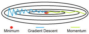
The graph to the right shows a comparison of gradient descent with and without momentum. Using momentum, the oscillations are significantly reduced and convergence to the minimum is achieved in fewer iterations.
Numerical Example
To demonstrate the use of momentum in the context of gradient descent, minimize the following function:
$ y=0.3*x^4 - 0.1*x^3 - 2*x^2 - 0.8*x $
SGD without Momentum
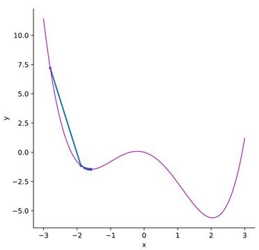
Solving this objective function using stochastic gradient descent, starting at x=-2.8 and a learning rate of 0.05, gives a solution of y=-1.46 and x=-1.59. This example uses python to construct a loss function and optimizer with PyTorch[6]. The following graph depicts how the stochastic gradient descent problem will stop at a local minimum instead of finding the global minimum of the function. The magenta line represents the objective function and the blue line shows the points at each iteration.

SGD with Momentum
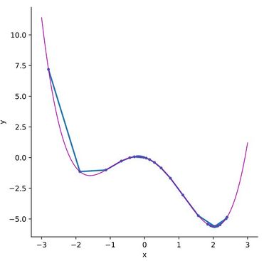
By adding momentum, the solver is able to overcome the hill past the local minimum and settle in the global maximum. The following example uses a momentum value of 0.7 and the same parameters as the previous example, with learning rate of 0.05 and starting point of x=2.8. Note that momentum values less than 0.7 are too low and are unable to overcome the hill past the local minimum. Using momentum, this solver gives the correct solution for the global minimum at y=-5.61 and x=2.04, shown in the graph below. The following table lists the values for x and y for each iteration after starting at x=-2.8.
| x | y | |
|---|---|---|
| 1 | -2.800 | 7.194 |
| 2 | -1.885 | -1.140 |
| 3 | -1.126 | -1.011 |
| 4 | -0.676 | -0.279 |
| ... | ... | |
| 99 | 2.042 | -5.608 |

Applications
Momentum is widely used in the machine learning community for training non-convex models such as deep neural networks[4]. Empirically, momentum methods outperform traditional stochastic gradient descent approaches[4]. The momentum extension for optimization algorithms is available in many popular machine learning frameworks such as pytorch, tensor flow, and scikit-learn.
Conclusion
hi
References
- ↑ 1.0 1.1 1.2 https://machinelearningmastery.com/gradient-descent-with-momentum-from-scratch/
- ↑ 2.0 2.1 https://towardsdatascience.com/gradient-descent-with-momentum-59420f626c8f
- ↑ Murphy, Kevin. Machine Learning. https://eds-p-ebscohost-com.proxy.library.cornell.edu/eds/ebookviewer/ebook/bmxlYmtfXzQ4MDk2OF9fQU41?sid=d9abaf85-26da-4cc7-87fc-020b7509ddf7@redis&vid=0&format=EB&rid=1
- ↑ 4.0 4.1 4.2 https://arxiv.org/pdf/2010.00406.pdf
- ↑ https://cedar.buffalo.edu/~srihari/CSE676/8.3%20BasicOptimizn.pdf
- ↑ PyTorch Tutorials. https://pytorch.org/tutorials/beginner/basics/optimization_tutorial.html