Momentum
Authors: Thomas Lee, Greta Gasswint, and Elizabeth Henning (SYSEN5800 Fall 2021)
Introduction
Momentum is an extension to the gradient descent optimization algorithm that builds inertia in a search direction to overcome local minima and oscillation of noisy gradients.[1] It is based on the same concept of momentum in physics. A classical example of the concept is a ball rolling down a hill that gathers enough momentum to overcome a plateau region and make it to a global minima instead of getting stuck at a local minima. Momentum adds history to the parameter updates of descent problems which significantly accelerates the optimization process. The amount of history included in the update equation is determined via a hyperparameter.[1] This hyperparameter is a value ranging from 0 to 1, where a momentum value of 0 is equivalent to gradient descent without momentum.[1] A higher momentum value means more gradients from the past (history) are considered.[2]
Gradient descent also has several limitations which can be addressed using momentum application, including issues with noise in the oscillations and potential failure to solve due to non-convex functions having multiple local minima.[3][2] Momentum addresses these limitations using exponentially weighted gradients, avoiding errors caused by iterations being equally weighted.
Theory, methodology, and/or algorithmic discussions
Algorithm
The main idea behind momentum is to compute an exponentially weighted average of the gradients and use that to update the weights. By taking past gradients into account, the steps to gradient descent become smoothed out, which can reduce the amount of oscillations seen in iterations (where the iterative solutions are going between above and below the true curve). [4]
In (stochastic) gradient descent without momentum, the update rule at each iteration is given by:
$ \theta_i=\theta_{i-1}-\gamma*g_i $
Where:
- $ \theta $ denotes the parameters to the cost function
- $ g_i $ is the gradient indicating which direction to decrease the cost function by
- $ \gamma $ is the hyperparameter representing the learning rate
In (stochastic) gradient descent with momentum, the update rule at each iteration is given by:
$ b_i=\mu*b_{i-1}+g_i $
$ \theta_i=\theta_{i-1}-\gamma*b_i $
Where:
- $ \theta $ denotes the parameters to the cost function
- $ g_i $ is the gradient indicating which direction to decrease the cost function by
- $ \gamma $ is the hyperparameter representing the learning rate
- $ b_i $ is the modified step direction term (as opposed to just using $ g_i $) that incorporates momentum
- $ \mu $ is a new hyperparameter that denotes the momentum constant
Momentum can be applied to other gradient descent variations such as batch gradient descent and mini-batch gradient descent. Regardless of the gradient descent variation, the momentum hyperparameter $ \mu $ must be tuned in addition to the learning rate hyperparameter $ \gamma $. $ \mu $ can be any value between 0 and 1. Generally, the larger the momentum value, the more past gradients must be taken into account, resulting in a smoother update. However, choosing a $ \mu $ value that is too large will result in over smoothing. It is also possible for a large $ \mu $ value to overshoot the target. As the $ \mu $ value gets closer to 0, momentum behaves similarly to steepest descent.[5] A value of 0 is essentially gradient descent without momentum and a momentum value of 0.9 tends to be a good default choice.[6] Finding the optimal $ \mu $ is a matter of trial and error to determine the best choice for a particular model such that the cost function is minimized.
Problems with Gradient Descent
With gradient descent, a weight update at time t is given by the learning rate and gradient at that exact moment.[2] This means that the previous steps are not considered when searching for the next iteration's solution.

This results in two issues:
- Unlike convex functions, a non-convex cost function can have many local minima's meaning the first local minima found is not guaranteed to be the global minima. At the local minima, the gradient of the cost function will be very small resulting in no weight updates. Because of this, gradient descent will get stuck and fail to find the global optimal solution.
- Gradient descent can be noisy with many oscillations which results in a larger number of iterations needed to reach convergence.[3]
Momentum is able to solve both of these issues buy using an exponentially weighted average of the gradients to update the weights at each iteration. This method also prevents gradients of previous iterations to be weighted equally. With an exponential weighted average, recent gradients are given more weight than previous gradients.
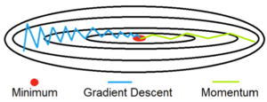
The graph to the right shows a comparison of gradient descent with and without momentum. Using momentum, the oscillations are significantly reduced and convergence to the minimum is achieved in fewer iterations.[7]
Numerical Example
To demonstrate the use of momentum in the context of gradient descent, minimize the following function:
$ y=0.3*x^4 - 0.1*x^3 - 2*x^2 - 0.8*x $
SGD without Momentum

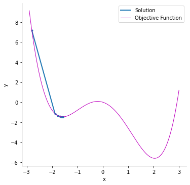
Solving this objective function using stochastic gradient descent, starting at $ \theta_0=-2.8 $ and a learning rate of $ \gamma=0.05 $, gives a final solution of $ x=-1.59 $ and $ y=-1.46 $. This example uses python to construct a loss function and optimizer with PyTorch.[8] The solver iterates through the following equations:
$ g_i = \nabla\theta_i f_i (\theta_{i-1}) = 1.2*\theta_{i-1}^3 - 0.3*\theta_{i-1}^2 - 4*\theta_{i-1} - 0.8 $
$ \theta_i=\theta_{i-1}-\gamma*g_i $
| Iteration | $ g_i $ | $ \theta_i $ |
|---|---|---|
| 1 | -18.294399999999 | -1.885279999999999 |
| 2 | -2.3661413363687 | -1.766972933181563 |
| 3 | -1.2889636339668 | -1.702524751483223 |
| 4 | -0.78138469777962 | -1.663455516594242 |
The graph to the right depicts how the stochastic gradient descent problem will stop at a local minimum instead of finding the global minimum of the function. The magenta line represents the objective function and the blue line shows the points at each iteration. The following table lists the solution values for $ x $ and $ y $ for each iteration.
| x | y | |
|---|---|---|
| 1 | -2.800 | 7.194 |
| 2 | -1.885 | -1.140 |
| 3 | -1.766 | -1.354 |
| 4 | -1.702 | -1.421 |
| 5 | -1.663 | -1.446 |
| ... | ... | |
| 99 | -1.586 | -1.464 |
SGD with Momentum

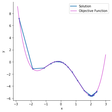
By adding momentum, the solver is able to overcome the hill past the local minimum and settle in the global maximum. The following example uses a momentum value of $ \mu=0.7 $ and the same parameters as the previous example, with learning rate of $ \gamma=0.05 $ and starting point of $ \theta_0=-2.8 $. The solver iterates through the following equations:
$ g_i = \nabla\theta_i f_i (\theta_{i-1}) = 1.2*\theta_{i-1}^3 - 0.3*\theta_{i-1}^2 - 4*\theta_{i-1} - 0.8 $
$ b_i=\mu*b_{i-1}+*g_i $
$ \theta_i=\theta_{i-1}-\gamma*b_i $
The values of $ b_i $ use momentum and information from previous iterations. For the first iteration, $ b_0=0 $. Therefore, the first iteration will have the same solution as the example without momentum.
| Iteration | $ g_i $ | $ b_i $ | $ \theta_i $ |
|---|---|---|---|
| 1 | -18.29439999999999 | 0 | -1.88527999999999 |
| 2 | -2.366141336368740 | -15.1722213363687 | -1.12666893318156 |
| 3 | 1.609651754221803 | -9.01090318123631 | -0.67612377411974 |
| 4 | 1.396449498127179 | -9.22410543733093 | -0.21491850225320 |
Note that momentum values less than 0.7 are too low and are unable to overcome the hill past the local minimum. The following table lists the values for $ x $ and $ y $ for each iteration after starting at $ \theta_0=-2.8 $. Using momentum, this solver gives the correct solution for the global minimum at $ x=2.04 $ and $ y=-5.61 $, as shown in the graph.
| x | y | |
|---|---|---|
| 1 | -2.800 | 7.194 |
| 2 | -1.885 | -1.140 |
| 3 | -1.126 | -1.011 |
| 4 | -0.676 | -0.279 |
| 5 | -0.431 | -0.008 |
| ... | ... | |
| 99 | 2.042 | -5.608 |
Applications
Momentum is widely used in the machine learning community for optimizing non-convex functions such as deep neural networks.[6] Empirically, momentum methods outperform traditional stochastic gradient descent approaches.[6] In deep learning, SGD is widely prevalent and is the underlying basis for many optimizers such as Adam, Adadelta, RMSProp, etc. which already utilize momentum to reduce computation speed.[9] The momentum extension for optimization algorithms is available in many popular machine learning frameworks such as PyTorch, tensor flow, and scikit-learn. Generally, any problem that can be solved with stochastic gradient descent can benefit from the application of momentum. These are often unconstrained optimization problems. Some common SGD applications where momentum may be applied are ridge and logistic regression and support vector machines.[10] Classification problems including those relating to cancer diagnosis[11] and image determination [12] can also have reduced run times when momentum is implemented. In the case of medical diagnoses, this increased computation speed can directly benefit patients through faster diagnosis times and higher accuracy of diagnosis within the neural network.
Momentum is also very useful in objective functions that have a large amount of curvature.[1] These are areas where the gradients changes a lot. Since momentum leverages an exponential weighted average, smaller steps will be taken in these regions that have higher curvature resulting in dampened oscillations.
Overall, momentum may have farther reaching applicability to accelerating second order methods and deeper connections to other methods, such as the ellipsoid algorithm.[13]
Conclusion
Momentum improves on gradient descent by reducing oscillatory effects and acting as an accelerator for optimization problem solving. Additionally, it finds the global (and not just local) optimum. Because of these advantages, momentum is commonly used in machine learning and has broad applications to all optimizers through SGD. Though the hyperparameters for momentum must be chosen with care and requires some trial and error, it ultimately addresses common issues seen in gradient descent problems. As deep learning continues to advance, momentum application will allow models and problems to be trained and solved faster than methods without.
References
- ↑ 1.0 1.1 1.2 1.3 Brownlee, J. (2021, October 11). Gradient descent with momentum from scratch. Machine Learning Mastery. https://machinelearningmastery.com/gradient-descent-with-momentum-from-scratch/.
- ↑ 2.0 2.1 2.2 Bhat, R. (2020, October 22). Gradient descent with momentum. Medium. https://towardsdatascience.com/gradient-descent-with-momentum-59420f626c8f
- ↑ 3.0 3.1 J. Sum, C. -S. Leung and K. Ho, "A Limitation of Gradient Descent Learning," in IEEE Transactions on Neural Networks and Learning Systems, vol. 31, no. 6, pp. 2227-2232, June 2020, doi: 10.1109/TNNLS.2019.2927689.
- ↑ Kevin P. Murphy. Machine Learning : A Probabilistic Perspective. The MIT Press; 2012. https://search-ebscohost-com.proxy.library.cornell.edu/login.aspx?direct=true&db=nlebk&AN=480968&site=ehost-live
- ↑ Craven, M., & Page, D. (n.d.). Deep learning II: Momentum & Adaptive Step Size - UW–madison. https://www.biostat.wisc.edu/~craven/cs760/lectures/DNNs-2.pdf
- ↑ 6.0 6.1 6.2 Defazio, A. Momentum via primal averaging: Theoretical Insights and Learning Rate Schedules for Non-Convex Optimization. https://arxiv.org/pdf/2010.00406.pdf
- ↑ 7.0 7.1 Srihari, S. (n.d.). Basic Optimization Algorithms. Deep learning.https://cedar.buffalo.edu/~srihari/CSE676/8.3%20BasicOptimizn.pdf
- ↑ PyTorch Tutorials. https://pytorch.org/tutorials/beginner/basics/optimization_tutorial.html
- ↑ Rosebrock, A. (2021, May 7). Gradient descent algorithms and variations. PyImageSearch. https://www.pyimagesearch.com/2021/05/05/gradient-descent-algorithms-and-variations/
- ↑ Menon, A. (2009, February 27). Large-Scale Support Vector Machines: Algorithms and Theory. https://cseweb.ucsd.edu//~akmenon/ResearchExamTalk.pdf
- ↑ Rehman, M. Z., & Nawi, N. M. (2011, June). The effect of adaptive momentum in improving the accuracy of gradient descent back propagation algorithm on classification problems. In International Conference on Software Engineering and Computer Systems (pp. 380-390). Springer, Berlin, Heidelberg.
- ↑ Zhang M., Smart W. (2004) Genetic Programming with Gradient Descent Search for Multiclass Object Classification. In: Keijzer M., O’Reilly UM., Lucas S., Costa E., Soule T. (eds) Genetic Programming. EuroGP 2004. Lecture Notes in Computer Science, vol 3003. Springer, Berlin, Heidelberg. https://doi.org/10.1007/978-3-540-24650-3_38
- ↑ Goh, G. (2017, April 4). Why momentum really works. Distill. https://distill.pub/2017/momentum/