Frank-Wolfe

Author: Adeline Tse, Jeff Cheung, Tucker Barrett (SYSEN 5800 Fall 2021)

Introduction

The Frank-Wolfe algorithm is an iterative first-order optimization algorithm for constrained convex optimization, first proposed by Marguerite Frank and Philip Wolfe from Princeton University in 1956. It is also known as the “gradient and interpolation” algorithm or sometimes the “conditional gradient method” as it utilizes a simplex method of comparing an initial feasible point with a secondary basic feasible point to maximize the linear constraints in each iteration to find or approximate the optimal solution.

Advantages of the Frank-Wolfe algorithm include that it is simple to implement, it results in a projection-free computation (that is, it does not require projections back to the constraint set to ensure feasibility), and it generates solution iterations that are sparse with respect to the constraint set. However, one of the major drawbacks of Frank-Wolfe algorithm is the practical convergence, which can potentially be an extremely slow computation process. Nonetheless, new sub-method has been proposed to accelerate the algorithm by better aligning the descent direction while still preserving the projection-free property. Therefore, despite the downside of Frank-Wolfe algorithm, the numerous benefits of this algorithm allow it to be utilized in artificial intelligence, machine learning, traffic assignment, signal processing, and many more applications.

Theory & Methodology

Figure 1. The Frank-Wolfe method optimizes by considering the linearization of the objective function f and moving the initial position x towards the minimizer of the linear function.

The Frank-Wolfe algorithm uses step size and postulated convexity, which formulates a matrix of positive semidefinite quadratic form. Just like a convex function yields a global minimum at any local minimum on a convex set, by the definition of nonlinear programming, the concave quadratic function would yield a global maximum point at any local maximum on a convex constraint set.

The methodology of the Frank-Wolfe algorithm starts with obtaining the generalized Lagrange multipliers for a quadratic problem, PI. The found multipliers are considered solutions to a new quadratic problem,  PII. The simplex method is then applied to the new problem, PII, and the gradient and interpolation method is utilized to make incremental steps towards the solution of the original quadratic problem, PI. This is performed by taking an initial feasible point, obtaining a second basic feasible point along the gradient of the objective function at the initial point, and maximizing the objective function along the segment that joins these two points.  The found maximum along the segment is utilized as the starting point for the next iteration. Using this method, the values of the objective function converge to zero and in one of the iterations, a secondary point will yield a solution.

Proof

• $X$ is a $[n\times 1]$ matrix
• $A$ is a $[m\times n]$ matrix
• $C$ is a $[n\times n]$ matrix
• $p$ and $b$ are $[1\times n]$ and $[1\times m]$ matrices respectively
• $\nabla f(x)$ is the gradient

$$f(x)=\sum _{j=1}^{n}p_{j}x_{j}-\sum _{j,k=1}^{n,n}X_{j}C_{jk}X_{k}$$

$$where\;\sum _{j=1}^{n}A_{ij}X_{j}\leq b_{i}\quad (i=1,...,m)\;and\;X_{j}\geq 0\quad (j=1,...,n)$$

$$\nabla f(x)={\frac {df(x)}{dx}}$$

PI is represented by the following equations using matrix notation:

$${\text{Maximize}}\qquad f(x)=px'-x'Cx\quad {\text{subject to}}$$

$$(I)={\begin{cases}x\geq 0\\Ax\leq b\end{cases}}$$

Since PI is feasible, any local maximum found that is contained within the convex constraint set is a global maximum. Then by utilizing Kuhn and Tucker's generalizations of the Lagrange Multipliers of the maximization of the objective function $f(x)$, $x_{0}$ is considered the solution of PI.

$$\delta f(x_{0})x_{0}=Max\,[\,\delta f(x_{0})w\,|\,w\geq 0,Aw\leq b],\quad where\;w\;{\text{is an}}\;[n\times 1]\;{\text{matrix}}$$

By the Duality Theorem,

$$Min\,[\,ub\,|\,u\geq 0,\,uA\geq \delta f(x_{o})],\quad where\;u\;{\text{is a}}\;[1\times m]\;{\text{matrix}}$$

Therefore, the solution $x_{0}$ for PI is only valid if:

$$Max\,[\,\delta f(x_{0})x_{0}-ub\,|\,u\geq 0,uA\geq \delta f(x_{0})]=0$$

Since

$$\delta f(x)=p-2x'Cx$$

Therefore, by the generalization of Lagrangian, $g(x,u)$ is extracted with linear constraints:

$$g(x,u)=\delta f(x)x-ub=px-ub-2x'Cx$$

$${\begin{cases}x\geq 0,\quad u\geq 0,\\Ax\leq b,\quad \delta f(x)\leq uA\end{cases}}$$

The completion of the generalized Lagrangian shows that $m+n$ positive variables exist for PI, thus a feasible solution exists.

Based on the concavity of $f$,

$$f(y)-f(x)\leq \delta f(x)(y-x)$$

If $(x,u)$ satisfies $g(x,u)\leq 0$ (where x is a solution if for some $u,\;g(x,u)=0$), then

$$f(y)-f(x)\leq \delta f(x)x\leq uAy-\delta f(x)x\leq ub-\delta f(x)x=-g(x,u)$$

By the Boundedness Criterion and the Approximation Criterion,

$$f(y)-f(x)\leq -g(x,u)$$

The Frank-Wolfe algorithm then adds a non-negative variable to each of the inequalities to obtain the following:

• $y$ and $\nu$ are $[m\times 1]$ and $[n\times 1]$ matrices respectively

$$x,\,u,\,y,\,\nu \geq 0$$

$$Ax+y=b$$

$$2Cx+A'u'-\nu '=p'$$

$$g(x,u)=\delta f(x)x-ub=(uA-\nu )x-u(Ax+y)=-\nu x+uy$$

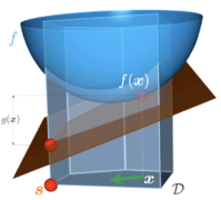
Thus, the PII problem is to obtain search vectors to satisfy $\nu x+uy=0$, and $x$ is considered a solution of PI if $\delta f(x)$ belongs to the convex cone spanned by the outward normals to the bounding hyperplanes on which $x$ lines as shown in Figure 1.

Algorithm

The Frank-Wolfe algorithm can generally be broken down into five steps as described below. Then the loop of iterations continues throughout Steps 2 to 5 until the minimum extreme point is identified.

Step 1. Define initial solution

If $x$ is the extreme point, the initial arbitrary basic feasible solution can be considered as:

$$x_{k}\in S\quad where\quad k=0$$

The letter $k$ denotes the number of iterations.

Step 2. Determine search direction

Search direction, that is the direction vector is:

$$p_{k}=y_{k}-x_{k}$$

$x_{k}$ and $y_{k}$ are feasible extreme points and belong to $S$ where $S$ is convex

First-order Taylor expansion around $x_{k}$ and problem is now reformulated to LP:

$${\begin{aligned}minimizes\quad &z_{k}(y)=f(x_{k})+\nabla f(x_{k})^{T}(y-x_{k})\\such\;that\quad &y\in S\\\end{aligned}}$$

Step 3. Determine step length

Step size $\alpha _{k}$ is defined by the following formula where $\alpha _{k}$ must be less than 1 to be feasible:

$$f(x_{k}+\alpha _{k}p_{k})<f(x_{k})$$

$$minimize_{\alpha \in [0,1]}\,f(x_{k}+\alpha p_{k})$$

Step 4. Set new iteration point

$$x_{k+1}=x_{k}+\alpha p_{k}$$

Step 5. Stopping criterion

Check if $x_{k+1}$ is an approximation of $x$, the extreme point. Otherwise, set $k=k+1$ and return to Step 2 for the next iteration.

In the Frank-Wolfe algorithm, the value of $f$ descends after each iteration and eventually decreases towards $f(x)$, the global minimum.

Numerical Example

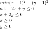
Consider the non-linear problem below.

Step 1. Choose a starting point

Begin by choosing the feasible point (0,0)

${\textstyle \delta fx(x,y)=2(x-1)=2x-2}$

${\textstyle \delta fy(x,y)=2(y-1)=2y-2}$

${\textstyle \nabla f(0,0)=z_{0}=[-2,-2]}$

Step 2. Determine a search direction The search direction is obtained by solving linear problem ${\textstyle \nabla f(0,0)\cdot (x,y)^{T}}$ subject to the constraints defined earlier The solution of this linear problem can be obtained via any linear programming algorithm, ie. enumeration with the feasible region's extreme points, the simplex method or GAMS. The solution to the linear problem is ${\textstyle (2,2)}$

The direction for this iteration ${\textstyle z_{0}}$ is found by ${\textstyle (x,y)^{T}-z_{0}}$ ${\textstyle [2,2]-[-2,-2]=[4,4]}$

The next point is found by ${\textstyle x_{1}=x_{0}+t*dir[0]}$ ${\textstyle x_{1}=x_{0}+t*[4,4]}$

Step 3. Determine Step Length We evaluate z(4t, 4t) to obtain t. ${\textstyle (4t-1)^{2}+(4t-1)^{2}=32t^{2}-16t+2}$ ${\textstyle \nabla f(t)=64t-16,t=16/64}$

Step 4. Set New Iteration Point Therefore ${\textstyle x_{1}=[0,0]+16/64*[4,4]=[1,1]}$

Step 5. Perform Optimality Test If the following equation yields a zero, the optimal solution has been found for the problem. ${\textstyle x_{1}=\nabla f(x_{0})*dir[0]}$ ${\textstyle x_{1}=\nabla f(x_{0})*dir[0]=-2*2+-2*2=-8}$

ITERATION 2

Step 1. Utilize new iteration point as the starting point ${\textstyle \nabla f(1,1)=z_{1}=(0,0)}$

At this point, because the gradient of the new starting point is [0,0], the optimality test will yield 0; therefore [1,1] is the optimum solution to the non-linear problem.

Conclusion

The Frank-Wolfe algorithm is one of the key techniques in the machine learning field. The algorithm features favor linear minimization, simple implementation, and low complexity. By using the simplex method that requires little alteration to the gradient and interpolation in each iteration, the optimization of the linearized quadratic objective function can be performed in a significantly shorter runtime and larger datasets can be processed more efficiently. Therefore, even though the convergence rate of Frank-Wolfe algorithm is slow due to the search for naive descent directions in each iteration, the benefits that the algorithm brings still outweigh the disadvantages. With the main characteristics of being projection-free and the capability of producing solutions for sparse structures, the algorithm gained popularity with many use cases in machine learning.

References

- ↑ 1.0 1.1 Frank, M. and Wolfe, P. (1956). An algorithm for quadratic programming. Naval Research Logistics Quarterly, 3(1-2):95–110.
- ↑ Combettes, C.W.. and Pokutta, S. (2020). Boosting Frank-Wolfe by chasing gradients. International Conference on Machine Learning (pp. 2111-2121). PMLR.
- ↑ Jaggi, M. (2013). Revisiting Frank-Wolfe: Projection-free sparse convex optimization. Inerational Conference on Machine Learning (pp.427-435). PMLR.
![{\displaystyle [n\times 1]}](https://wikimedia.org/api/rest_v1/media/math/render/svg/7b8626c8f96ac82b5c7770fde351ede0137e3992)
![{\displaystyle [m\times n]}](https://wikimedia.org/api/rest_v1/media/math/render/svg/60b617e206c9fb5fae1e89d73a33c75e826480c5)
![{\displaystyle [n\times n]}](https://wikimedia.org/api/rest_v1/media/math/render/svg/47fc57498a8040ee9d4117056a6663e0b165ec6f)
![{\displaystyle [1\times n]}](https://wikimedia.org/api/rest_v1/media/math/render/svg/2dc04bdc0bddba51eeca7eed8515ca35f1d79662)
![{\displaystyle [1\times m]}](https://wikimedia.org/api/rest_v1/media/math/render/svg/40df39f1cf3304969234e1835f02288e27e6599f)
![{\displaystyle \delta f(x_{0})x_{0}=Max\,[\,\delta f(x_{0})w\,|\,w\geq 0,Aw\leq b],\quad where\;w\;{\text{is an}}\;[n\times 1]\;{\text{matrix}}}](https://wikimedia.org/api/rest_v1/media/math/render/svg/e786b861c24421494b439bbaeac15880c021e682)
![{\displaystyle Min\,[\,ub\,|\,u\geq 0,\,uA\geq \delta f(x_{o})],\quad where\;u\;{\text{is a}}\;[1\times m]\;{\text{matrix}}}](https://wikimedia.org/api/rest_v1/media/math/render/svg/4355b9102d4d9a6d4d44fbd0c1e7c63c421d1495)
![{\displaystyle Max\,[\,\delta f(x_{0})x_{0}-ub\,|\,u\geq 0,uA\geq \delta f(x_{0})]=0}](https://wikimedia.org/api/rest_v1/media/math/render/svg/19b1fb7db0d7158b728e880c4009dbc7cc654fe3)
![{\displaystyle [m\times 1]}](https://wikimedia.org/api/rest_v1/media/math/render/svg/1fcc3d1a24030bca3afee3d5d4f892b108a2496c)
![{\displaystyle minimize_{\alpha \in [0,1]}\,f(x_{k}+\alpha p_{k})}](https://wikimedia.org/api/rest_v1/media/math/render/svg/3e53164c3ceec36747812ddc5f032fdb60932d15)
![{\textstyle \nabla f(0,0)=z_{0}=[-2,-2]}](https://wikimedia.org/api/rest_v1/media/math/render/svg/396bd05ed3270896af81ab3e15446c52ea70b0f8)
![{\textstyle [2,2]-[-2,-2]=[4,4]}](https://wikimedia.org/api/rest_v1/media/math/render/svg/5bc503d675157b9ee7284e4535d4897e19116ef3)
![{\textstyle x_{1}=x_{0}+t*dir[0]}](https://wikimedia.org/api/rest_v1/media/math/render/svg/d870d460185548efb9a1c99b1e685fd10b622298)
![{\textstyle x_{1}=x_{0}+t*[4,4]}](https://wikimedia.org/api/rest_v1/media/math/render/svg/2f56e6e3a6bd4acd11703c38126e02b4ff4043a3)
![{\textstyle x_{1}=[0,0]+16/64*[4,4]=[1,1]}](https://wikimedia.org/api/rest_v1/media/math/render/svg/e96123b84177708c4cab3af1656b4463999de361)
![{\textstyle x_{1}=\nabla f(x_{0})*dir[0]}](https://wikimedia.org/api/rest_v1/media/math/render/svg/9aeae691a0df3daad79cf7e688739761290228ca)
![{\textstyle x_{1}=\nabla f(x_{0})*dir[0]=-2*2+-2*2=-8}](https://wikimedia.org/api/rest_v1/media/math/render/svg/be2497585b8f6dd1b467084c3b2931c91025ac4e)