Momentum

Authors: Thomas Lee, Greta Gasswint, Elizabeth Henning (SYSEN5800 Fall 2021)

Introduction

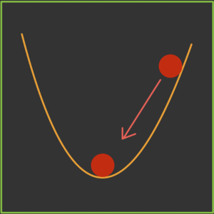
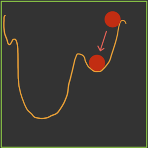
Momentum is an extension to the gradient descent optimization algorithm that builds inertia in a search direction to overcome local minima and oscillation of noisy gradients. It is based on the same concept of momentum in physics. A classic example is a ball rolling down a hill that gathers enough momentum to overcome a plateau region and make it to a global minima instead of getting stuck at a local minima. Momentum adds history to the parameter updates which significantly accelerates the optimization process. Momentum controls the amount of history to include in the update equation via a hyperparameter. This hyperparameter is a value ranging from 0 to 1. A momentum of 0 is equivalent to gradient descent without momentum. A higher momentum value means more gradients from the past (history) are considered.

Theory, methodology, and/or algorithmic discussions

Definition

hi

Algorithm

The main idea behind momentum is to compute an exponentially weighted average of the gradients and use that to update the weights. By taking past gradients into account, the steps to gradient descent become smoothed out.

In gradient descent (stochastic) without momentum, the update rule at each iteration is given by:

W = W - $\alpha$dW

Where:

• W denotes the parameters to the cost function
• dW is the gradient indicating which direction to decrease the cost function by
• $\alpha$ is the hyperparameter representing the learning rate

In gradient descent (stochastic) with momentum, the update rule at each iteration is given by:

V$dw$ = βV$dw$ + (1-β)dW

W = W - $\alpha$V$dw$

Where:

• β is a new hyperparameter that denotes the momentum constant

Momentum can be applied to other gradient descent variations such as batch gradient descent and mini-batch gradient descent. Regardless of the gradient descent variation, the momentum hyperparameter β will need to be tuned in addition to the learning rate hyper parameter $\alpha$. β can be any value between 0 and 1. Generally, the larger the momentum value, the more we take past gradients into account. This results in a smoother update. Consequently, choosing a β value that is too large will result in over smoothing. A momentum value of 0.9 tends to be a good default choice. Finding the optimal β is a matter of trial and error to see what works best for your model such that the cost function is minimized.

Problems with Gradient Descent

A gradient descent scenario for a convex cost function.

With gradient descent, a weight update at time t is given by the learning rate and gradient at that exact moment. It doesn't not consider previous steps when searching.

This results in two issues:

1. Unlike convex functions, a non-convex cost function can have many local minima's meaning the first local minima found is not guaranteed to be the global minima. At the local minima, the gradient of the cost function will be very small resulting in no weight updates. Because of this, gradient descent will get stuck and fail to find the most optimal solution.
2. Gradient descent can be noisy with many oscillations which results in a larger number of iterations needed to reach convergence.

Momentum is able to solve both of these issues but using an exponentially weighted average of the gradients to update the weights at each iteration. This method also prevents gradients of previous iterations to be weight equally. With an exponential weighted average, recent gradients are given more weightage than previous gradients. This can be seen in the numerical example below.

Another heading

hi

Another heading

hi

Graphical Explanation

A gradient descent scenario, without momentum, for a non-convex cost function.

hi

hi

hi

another header

• hi

another heading

• Blah:

Some Example

• More text

Numerical Example

To demonstrate the use of momentum in the context of gradient descent, minimize the following function:

$f(x)=0.1x_{1}^{2}+2x_{2}^{2}$

This is a very stretched ellipsoid objective function with a minimum at (0,0). The gradient in the direction of $x_{2}$ changes at a much faster rate than $x_{1}$ due to the stretched nature of this function. Using gradient descent without momentum presents a challenge for selecting a learning rate. A small learning rate guarantees convergence in the $x_{2}$direction, but will converge very slowly in the $x_{1}$ direction which is an issue. The alternative is a higher learning rate, which runs the risk of diverging in $x_{2}$but will converge much quicker in the $x_{1}$ direction. The following graph shows the steps for solving this problem using a learning rate of 0.4.

INSERT GRAPH HERE

Because the gradient is oscillating significantly in the above example, using momentum will be an effective way to reduce the time to reach the minimum. Momentum v at time t replaces the instantaneous gradient with a weighted value that is averaged recursively using the past gradients. The following shows the equations for solving this using momentum:

Failed to parse (syntax error): {\textstyle v_t = \beta\*v_{t-1} } gahhh why wont this equation work

INSERT GRAPH HERE

Applications

Momentum is widely used in the machine learning community for training non-convex models such as deep neural networks. Empirically, momentum methods outperform traditional stochastic gradient descent approaches. The momentum extension for optimization algorithms is available in many popular machine learning frameworks such as pytorch, tensor flow, and scikit-learn.

In backpropgation,

Conclusion

hi