RMSProp

Author: Jason Huang (SysEn 6800 Fall 2020)

Introduction

RMSProp, so call root mean square propagation, is an optimization algorithm/method designed for Artificial Neural Network (ANN) training. And it is an unpublished algorithm first proposed in the Coursera course “Neural Network for Machine Learning” lecture six by Geoff Hinton. RMSProp lies in the realm of adaptive learning rate methods, which have been growing in popularity in recent years because it is the extension of Stochastic Gradient Descent (SGD) algorithm, momentum method, and the foundation of  Adam algorithm. One of the applications of RMSProp is the stochastic technology for mini-batch gradient descent.

Theory and Methodology

Perceptron and Neural Networks

Perceptron is an algorithm used for supervised learning of binary classifier, and also can be regard as the simplify version/single layer of the Artificial Neural Network to better understanding the neural network, which is to perform the human brain and conscious center in Artificial Intelligence(AI) and presenting the imitation of what the mind will like when human thinking. The basis form of the perceptron consists inputs, weights, bias, net sum and activation function.

The process of the perceptron is start by initiating input value $x_{1},x_{2}$ and multiplying them by their weights to obtain $w_{1},w_{2}$. All of the weights will be added up together to create the weight sum$\sum _{i}w_{i}$. And the weighted sum is then applied to the activation function $f$ to produce the perceptron's output.

A single neuron presented as a mathematic function

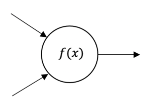
A neural network works similarly to the human brain’s neural network. A “neuron” in a neural network is a mathematical function that collects and classifies information according to a specific architecture. A neural network contains layers of interconnected nodes, which can be regards as the perception and is similar to the multiple linear regression. The perceptron transfers the signal by a multiple linear regression into an activation function which may be nonlinear.

RProp

RProp, or we call Resilient Back Propagation, is the widely used algorithm for supervised learning with multi-layered feed-forward networks in the past. The basic concept of the backpropagation learning algorithm � is the repeated application of the chain rule to compute the influence of each weight in the network with respect to an arbitrary error. The derivatives equation of error function can be represented as:

${\frac {\partial E}{\partial w_{ij}}}={\frac {\partial E}{\partial s_{i}}}{\frac {\partial s_{i}}{\partial net_{i}}}{\frac {\partial net_{i}}{\partial w_{ij}}}$

Where $w_{ij}$ is the weight from neuron $j$ to neuron $i$, $s_{i}$ is the output , and $net_{i}$ is the weighted sum of the inputs of neurons $i$. Once the weight of each partial derivatives is known, the error function can be presented by performing a simple gradient descent:

$w_{ij}(t+1)=w_{ij}(t)-\epsilon {\frac {\partial E}{\partial w_{ij}}}(t)$

The choice of the learning rate $\epsilon$, which scales the derivative, has an important effect on the time needed until convergence is reached. If it is set too small, too many steps are needed to reach an acceptable solution; on the contrary, a large learning rate will possibly lead to oscillation, preventing the error to fall below a certain value⁷.

In addition, RProp can combine the method with momentum method, to prevent above problem and to accelerate the convergence rate, the equation can rewrite as:

$\Delta w_{ij}(t)=\epsilon {\frac {\partial E}{\partial w_{ij}}}(t)+\mu \Delta w_{ij}(t-1)$

However, It turns out that the optimal value of the momentum parameter $\mu$ in above equation is equally problem dependent as the learning rate $\epsilon$, and that no general improvement can be accomplished. Besides, RProp algorithm is not function well when we have very large datasets and need to perform mini-batch weights updates. Therefore, scientist proposal a novel algorithm, RMSProp, which can cover more scenarios than RProp.

RMSProp

RProp algorithm does not work for mini-batches is because it violates the central idea behind stochastic gradient descent, which is when we have a small enough learning rate, it averages the gradients over successive mini-batches. To solve this issue, consider the weight, that gets the gradient 0.1 on nine mini-batches, and the gradient of -0.9 on tenths mini-batch, RMSProp did force those gradients to roughly cancel each other out, so that the stay approximately the same.

By using the sign of gradient from RProp algorithm, and the mini-batches efficiency, and averaging over mini-batches which allows combining gradients in the right way. RMSProp is keeping the moving average of the squared gradients for each weight. And then we divide the gradient by square root the mean square.

The updated equation can be performed as:

$E[g^{2}](t)=\beta E[g^{2}](t-1)+(1-\beta )({\frac {\partial c}{\partial w}})^{2}$

$w_{ij}(t)=w_{ij}(t-1)-{\frac {\eta }{\sqrt {E[g^{2}]}}}{\frac {\partial c}{\partial w_{ij}}}$

where $E[g]$ is the moving average of squared gradients, $\delta c/\delta w$ is gradient of the cost function with respect to the weight, $\eta$ is the learning rate and $\beta$ is moving average parameter (default value — 0.9, to make the sum of default gradient value 0.1 on nine mini-batches and -0.9 on tenths is approximate zero, and the default value $\eta$ is 0.001 as per experience).

Numerical Example

For the simple unconstrainted optimization problem $minf(x)=0.1x_{1}^{2}+2x_{2}^{2}$ :

settle $\beta$ = 0.9, $\eta$ = 0.4, , and transform the optimization problem to the standard RMSProp form, the equations are presented as below:

The visualization of the trajectory of RMSProp algorithm

${\frac {\partial c_{1}}{\partial w_{2}}},{\frac {\partial c_{2}}{\partial w_{2}}}=0.2x_{1},4x_{2}$

$E_{1}(t)=0.9E_{1}(t-1)+(1-0.9)({\frac {\partial c_{1}}{\partial w_{1}}})^{2}$

$E_{2}(t)=0.9E_{2}(t-1)+(1-0.9)({\frac {\partial c_{2}}{\partial w_{2}}})^{2}$

$w_{1}(t)=w_{1}(t-1)-{\frac {-0.4}{\sqrt {E_{1}}}}{\frac {\partial c_{1}}{\partial w_{1}}}$

$w_{2}(t)=w_{2}(t-1)-{\frac {-0.4}{\sqrt {E_{1}}}}{\frac {\partial c_{2}}{\partial w_{2}}}$

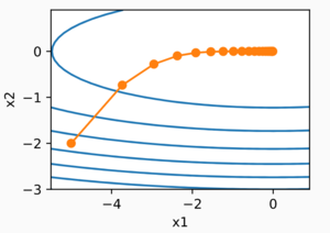
while using programming language to help us to visualize the trajectory of RMSProp algorithm, we can observe that the curve converge to a certain point.

Applications and Discussion

Visualizing Optimization algorithm comparing convergence with similar algorithm¹

Visualizing Optimization algorithm comparing convergence with similar algorithm¹

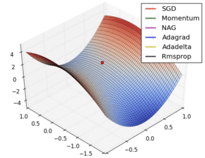
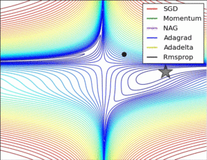
The applications of RMSprop concentrate on the optimization with complex function like the neural network, or the nonconvex optimization problem with adaptive learning rate, and widely used in the stochastic problem. The RMSprop optimizer restricts the oscillations in the vertical direction. Therefore, we can increase the learning rate and our algorithm could take larger steps in the horizontal direction converging faster than the similar approach gradient descent algorithm combine with momentum method.

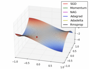
In the first visualization scheme, the gradients based optimization algorithm has a different convergence rate. As the visualizations are shown, without scaling based on gradient information algorithms are hard to break the symmetry and converge rapidly. RMSProp has a relative higher converge rate than SGD, Momentum, and NAG, beginning descent faster, but it is slower and Ada-grad, Ada-delta, which are the Adam based algorithm. In conclusion, when handling the large scale/gradients problem, the scale gradients/step sizes like Ada-delta, Ada-grad, and RMSProp perform better with high stability.

Ada-grad adaptive learning rate algorithms that look a lot like RMSProp. Ada-grad adds element-wise scaling of the gradient-based on the historical sum of squares in each dimension. This means that we keep a running sum of squared gradients, and then we adapt the learning rate by dividing it by the sum to get the result. Considering the concepts in RMSProp widely used in other machine learning algorithms, we can say that it has high potential to coupled with other methods such as momentum,...etc. To better increase the converge rate and accuracy.

Conclusion

RMSProp, root mean squared propagation is the optimization machine learning algorithm to train the Neural Network (NN) of Artificial Intelligence by different adaptive learning rate, derived from the concepts of gradients descent and RProp. Combining averaging over mini-batches and efficiency, and the gradients over successive mini-batches, RMSProp can reach the faster convergence rate than the original optimizer, but lower than the advanced optimizer such as Adam. As knowing the high performance of RMSProp, extensive implementation can be envisaged in the future.

Reference

1. Visualizing Optimization Algos

2. R Yamashita, M Nishio, R Kinh Gian, Convolutional neural networks: an overview and application in radiology (2018), 9:611–629

3. Vitaly Bushave, Understanding RMSprop — faster neural network learning (2018)

4. Vitaly Bushave, How do we ‘train’ neural networks ? (2017)

Visualizing Optimization algorithm comparing convergence with similar algorithm¹

5. Sebastian Ruder, An overview of gradient descent optimization algorithms (2016)

6. Rinat Maksutov, Deep study of a not very deep neural network. Part 3a: Optimizers overview (2018)

7. Martin Riedmiller, H Braun, A Direct Adaptive Method for Faster Backpropagation Learning: The RPROP Algorithm (1993) 586-591

8. Dario Garcia-Gasulla, An Out-of-the-box Full-network Embedding for Convolutional Neural Networks (2018) 168-175

9. Neural Networks for Machine Learning, Geoffrey Hinton

10. Python keras.optimizers.RMSprop() Examples

11. RMSProp Algorithm Implementation Example