Spatial branch and bound method

Authors: Ellen Zhuang (ChE 345 Spring 2015)
Steward: Dajun Yue, Fengqi You

Spatial branch-and-bound is a divide-and-conquer technique used to find the deterministic solution of global optimization problems.¹ It is a type of branch-and-bound method, which solves for the set of parameters that globally optimize the objective function, whether that be finding the minimum or maximum value of $f(x)$ or $-f(x)$, respectively, where x exists over a set of candidate solutions in the feasible region of the problem.

Introduction

Branch-and-bound is the systematic enumeration of possible solutions by iteratively searching the space of the problem. The problem’s candidate solutions form a rooted tree. The algorithm analyzes the nodes, or the subsets of the solution set. This step is known as branching. Bounding is the estimation of a lower and upper bound for the optimal solution at each node. The possible solution at each branch is checked against these bounds, and if it does not produce a better solution than the current best solution found, the solution is discarded in a step called pruning. This algorithm is repeated until the optimal solution is found. The method was first proposed by A. H. Land and A. G. Doig in 1960 for discrete programming, and its first applications were for discrete problems like the traveling salesman problem.

Spatial branch-and-bound techniques solve mixed integer nonlinear programs (MINLP) with nonconvex terms. Unlike ordinary branch-and-bound methods for mixed integer linear programs (MILP), the spatial branch-and-bound method decomposes the nonlinear functions of the original problem symbolically and recursively with simple operators into simple functions.³

Comparison of branch-and-bound for MILP and spatial branch-and-bound for nonconvex MINLP.

	Branch-and-bound for MILP	Spatial branch-and-bound for MINLP
Relaxation	replace integer variables with bounded continuous variables to form LP	replace nonconvex terms with their convex envelopes to form convex (MI)NLP
Branching	on integer variables	on integer and continuous variables
Complexity	NP-hard	NP-hard (but harder)

Spatial branch-and-bound is used to solve global optimization problems of the form:

$minf(x)$

$s.t.$ $g_{i}(x)\leq 0$ where $i=1,2,...,n$

$x\in S$

where S is the set of candidate solutions and is a union of the subsets $S_{j}$ where $j=1,2,...,n$. All functions $f(x)$ and $g_{i}(x)$ are at least continuously differentiable on some open set containing the subregion $S_{j}$ with bounds $s_{j}^{L}\leq x\leq s_{j}^{U}$, where $s_{j}^{L}$ and $s_{j}^{U}$ are the lower and upper bounds of $S_{j}$, respectively. The feasible space of the problem is where $x\in S$ and $g_{i}(x)\leq 0$. The goal is to find the point $x^{*}$ in the feasible region where $f^{*}(x)\leq f(x)+\epsilon$, where $\epsilon >0$ is a given tolerance.

Algorithm

The main algorithmic idea is to divide the problem into smaller subproblems by branching the variables into possible values, creating upper and lower bounds of the function in the certain domain, and finding sequences of approximate solutions which converge to the actual solution. The smaller subproblems are easier to solve than the original problem.²

Convex relaxation is performed on the original nonconvex problem and underestimates the optimal value of the original function. The original problem is then allocated in the root node of the tree. With each iteration, the original problem is restricted , and the subregions are relaxed to make convex.¹ For each subregion, the lower and upper bounds of the optimal value of the objective function is found. If the bounds converge, then the global optimum value to the subregion is found. If the bounds do not meet the desired tolerance, the problem is partitioned into smaller subproblems (descendants) by dividing the feasible space of continuous variable (branching variable). The two subproblems are solved by recursive partitioning. If the subproblem does not have the global optimal solution, then it is pruned. The process is continued until the global optimum value of the original problem is found.²

Convergence Proof

A branch and bound method using an exact selection rule will converge. Let M be the space of the sample. M is split at some iteration because it consists of an unqualified region that does not include candidate solutions that give the objective function more optimal solutions than the current incumbent solution. Thus, every qualified subregion of M_n contains the optimal solution.¹

It is noted that the spacial branch and bound algorithm does not guarantee convergence in a finite number of steps. The algorithm here uses the concept of ɛ-optimality instead of the usual idea of optimality. A solution x* is a global optimum if f(x*) < f(x) for x in the problem space. Because ɛ is positive, x^ɛ in the problem space is ɛ-globally optimal if the optimum is bounded by m ≤ f(x*) ≤ M where f(x^ɛ) is in [m,M] and M - m < ε. Finding the ε-global optimum solution ensures a finite termination than a usual global optimum solution.¹

Convergence is accelerated with fathoming. For each subregion, the lower bounding solution and the corresponding lower bounding objective function value are found. The region with the lowest objective function value is usually selected. An upper bound to the problem bounds the problem from above. It discards any region where the lower bound of the objective function exceeds the best upper bound. The discarded regions are fathomed.¹

Step 1: Initialization

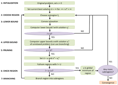
Initialize the subregions S_j to a single region S encompassing the set of all variables and their ranges. Set the convergence tolerance, ɛ > 0, and the best solution U = ∞ and the corresponding solution -∞ < x^* < ∞.

Step 2: Choice of Region

A subregion S_j of the problem is chosen.

Bound tightening may be performed during the first two steps. For the initialization step, optimization-based bounds tightening involves finding the smallest range of each variable subject to convex relaxation that will still make the problem feasible. This bounds tightening, however, is computationally expensive because 2n convex NLP or linear convex relation problems have to be solved, where n is the number of variables. For the second step, feasibility-based bounds tightening is performed at each region. Here, the variable bounds are tightened with the constraints of the original problem. This type of bounds tightening is computationally less expensive than the former. The spatial branch-and-bound algorithm will still converge without bound tightening, but it may make the process faster.

Step 3: Lower Bound

A convex relaxed problem of the original problem in the region chosen is formulated. The problem is reduced to standard form by linearizing the nonlinear terms. The nonlinear terms are replaced by added variables and constraints of type "added variable = nonlinear term". The nonconvex terms are also replaced by convex under- and over- estimators such as convex envelopes. Convex relaxation guarantees a lower bound to the objective function value in that region.

The new problem is solved to give an underestimation l of the objective function with solution x_j^L. If l > U , the relaxed problem is infeasible and step 2 is repeated.

Step 4: Upper Bound

Since the lower bound (LB) of S₂ is greater than the upper bound (UB) of S₁, which is the current best solution, so the solution in the region S₂ is infeasible and discarded.

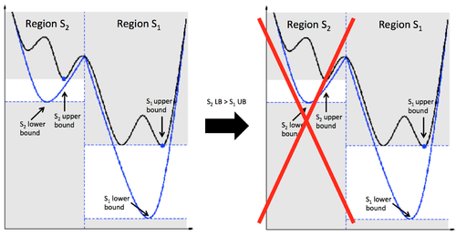
The original nonconvex problem in the selected region is solved to obtain a local optimum solution x_j^U with objective function u . The subproblem can be solved numerically or by branching. If the spatial branch-and-bound algorithm has added variables, branching can be done on those. Convex relaxation is done, and the lower and upper bounds are found. These bounds are not dependent on the added variables. Branching can also be done on the original variables. The range of the original problem [x^L, x^U] is partitioned into [x^L, x'] and [x', x^U]. The upper bounding problem is solved in each subregion.

Algorithms that solve nonconvex NLPs are fragile and can fail even if a local optimum solution exists. If the function is unable to be solved, set u = ∞ and -∞ < x_j^U < ∞.

Step 5: Pruning

If U > u , set x^* = x^U and U = u . All the regions with lower bounds greater than U are discarded.

Step 6: Check Region

If u - l ≤ ɛ, then u is a global minimum of the region, and the algorithm returns to step 2. If not, then the global minimum of the subregion is not found, and the algorithm proceeds to the next step.

Step 7: Branching

The region is split into sub-regions, and the algorithm returns to step 2. There are several strategies for branching, and most consist of determining the set of variables on which to branch and the variables whose domain is sub-divided by the branching operation.

Example¹

The global optimization problem min f(x) = 1/4 x + sin(x).¹

$min$ $f(x)$ $=1/4x+$$sin(x)$

$s.t.$ $-3\leq x\leq 6$

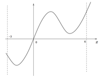
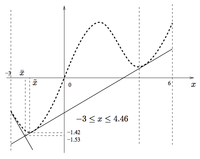
The above NLP has two minima, one of which is global. Using the spatial branch-and-bound approach, the space of the problem is divided into subregions, within which the lower and upper bounds of the optimum is found. If the bounds are not within a given $\epsilon <0$ tolerance (that is, the bounds are not sufficiently close), then the subregion is partitioned and the process is repeated. In this example, let $\epsilon =0.15$.

First Iteration

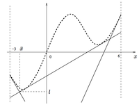
Consider the region that encompasses the entire range $-3\leq x\leq 6$. The objective function is underestimated with the convex underestimator $1/4x-1$. To tighten the bounds, tangents to $f(x)$ are added:

$-0.74x-3.11$ at $x=-3$

$1.21x-6.04$ at $x=6$.

The convex estimator is then $f^{c}(x)=\{-0.74x-3.11,1/4x-1,1.21x-6.04\}$.

The minimum of the convex problem is found to be $l=-1.53$ at $x^{L}=-2.13$.

Next, the upper bound of the problem is solved locally using Newton's method with $x=6$ as the starting point. The upper bound is found to be $u=0.147$ at $x^{U}=4.46$. $u$ and $l$ are not sufficiently close since $u-l=1.67>1$, so it is not certain that $x^{U}$ is a global optimum of the region.

The region is partitioned into two subregions, using $x^{U}=4.46$ as the branching point. The two unexamined regions are now $-3\leq x\leq 4.46$ and $4.46\leq x\leq 6$.

The convex relaxation and lower bound of the first region examined.¹

Second Iteration

Here, let $-3\leq x\leq 4.46$ be the first region to be examined. The lower and upper bounds are found to be $l=-1.53$ (as before) and $u=-1.43$ at $x^{U}=-1.823$. Now, $u-l=0.11<\epsilon$, so $x^{U}=-1.823$ is accepted as the global optimum of the region analyzed. The best solution found thus far is now $x^{*}=-1.823$ and $U=-1.42$. Since a global optimum exists, the region does not need to be branched.

The second iteration.¹

Third Iteration

The region $4.46\leq x\leq 6$ is examined. The lower and upper bounds are computed to be $l=1.11$ at $x^{L}=4.46$ and $u=1.147$ at $x^{U}=4.46$. Since $u-l=0.04<\epsilon$, the solution found is the optimum of the subregion, and branching is not necessary. The best solution found thus far does not need to be updated since $U<u$, so this region is discarded. The algorithm converges at the global optimum $x^{*}=-1.823$.

The third iteration.¹

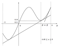
This example illustrates important features of the spatial branch-and-bound approach. First, the convex relaxation can be made tighter in each region. Second, in problems with multiple variables, the choice of the variable on which to branch is important. Third, the subregions are pruned when its lower bound is higher than the best solution found thus far.

Applications

Spatial branch-and-bound is used to solve a number of problems, including

• Pooling and Blending Problems: An example of a pooling/blending problem is the mixing of various types of crude oils with different qualities from different feeds. These streams are mixed in various pools. The parameters of the mixing are set to minimize cost while meeting quality requirement and quantity demand.
• Euclidean Location Problems: An example of this problem is finding the geographical positions of a plant that minimizes transportation costs.
• Kissing Number Problem: The objective of the kissing number problem is to find the maximum number of non-overlapping n-dimensional spheres in (n+1)-dimensional Euclidian space that can be arranged such that each is touching another. In 1-dimension, the kissing number is 2; in 2-dimension, 6; and in 3-dimension, 12.

Conclusion

Accurate models of real problems often involve nonconvex terms in either the objective function or the constraints. Nonconvex problems are one of the hardest to solve. Since there are multiple local optima solutions, it is difficult to find which solution is the best. Global optimization approaches, such as spatial branch-and-bound, are used to solve such problems. Other algorithms have been derived from the original spatial branch-and-bound. Examples include branch-and-reduce, α branch-and-bound, symbolic reformulation, branch-and-contract, and reduced spatial branch-and-bound.

References

1. Liberti, Leo. "Introduction to global optimization." Lecture of Ecole Polytechnique, Palaiseau F 91128 (2008): 12.
2. Pozo, C., et al. "A spatial branch-and-bound framework for the global optimization of kinetic models of metabolic networks." Industrial & Engineering Chemistry Research 50.9 (2010): 5225-5238.
3. Stein, Oliver, Peter Kirst, and Paul Steuermann. "An Enhanced Spatial Branch-and-Bound Method in Global Optimization with Nonconvex Constraints." (2013).