Trust-region methods: Difference between revisions
| Line 3: | Line 3: | ||
=Problem formulation= | =Problem formulation= | ||
=Numerical example= | =Numerical example= | ||
Here we will use the trust-region method to solve a classic optimization problem, the Rosenbrock function. The Rosenbrock function is a non-convex function, introduced by Howard H. Rosenbrock in 1960, which is often used as a performance test problem for optimization algorithms. This problem is solved using MATLAB's fminunc as the solver, with 'trust-region' as the solving algorithm. | Here we will use the trust-region method to solve a classic optimization problem, the Rosenbrock function. The Rosenbrock function is a non-convex function, introduced by Howard H. Rosenbrock in 1960, which is often used as a performance test problem for optimization algorithms. This problem is solved using MATLAB's fminunc as the solver, with 'trust-region' as the solving algorithm which uses the preconditioned conjugate method. | ||
The function is defined by | The function is defined by | ||
| Line 11: | Line 11: | ||
The starting point chosen is <math>x=0</math> <math>y=0 | The starting point chosen is <math>x=0</math> <math>y=0 | ||
</math>. | </math>. | ||
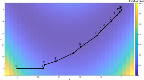
[[File:TRM Trajectory.jpg|thumb|565x565px|Optimization trajectory of the example]] | |||
'''Iteration Process''' | '''Iteration Process''' | ||
'''Iteration 1:''' | '''Iteration 1:''' The algorithm starts from the initial point of <math>x=0</math>, <math>y=0 | ||
</math>. The Rosenbrock function is visualized with a color coded map. For the first iteration, a full step was taken and the optimal solution (<math>x=0.25</math>, <math>y=0 | |||
</math>) within the trust-region is denoted as a red dot. For each consecutive iteration, | |||
'''Iteration 2:''' Start with '''<math>x=0.263177536 | |||
</math>, <math>y=0.061095029 | |||
</math>''' | |||
'''Iteration 3:''' Start with <math>x=0.371151679 | |||
</math>, <math>y=0.124075855 | |||
</math> | |||
'''Iteration 4:''' Start with '''<math>x=0.539493472 | |||
</math>, <math>y=0.262714248 | |||
</math>''' | |||
'''Iteration 5:''' Start with '''<math>x=0.608557768 | |||
</math>, <math>y=0.36557268 | |||
</math>''' | |||
... | |||
At the 16th iteration, the global optimal solution is found, '''<math>x=1 | |||
</math>, <math>y=1 | |||
</math>''' | |||
{| class="wikitable" | {| class="wikitable" | ||
Revision as of 01:47, 27 November 2021
Autor: Chun-Yu Chou (cc2398), Ting Guang Yeh (ty262), Yun-Chung Pan (yp392), Chen-Hua Wang (cw893), Fall 2021
Introduction
Problem formulation
Numerical example
Here we will use the trust-region method to solve a classic optimization problem, the Rosenbrock function. The Rosenbrock function is a non-convex function, introduced by Howard H. Rosenbrock in 1960, which is often used as a performance test problem for optimization algorithms. This problem is solved using MATLAB's fminunc as the solver, with 'trust-region' as the solving algorithm which uses the preconditioned conjugate method.
The function is defined by
The starting point chosen is .

Iteration Process
Iteration 1: The algorithm starts from the initial point of , . The Rosenbrock function is visualized with a color coded map. For the first iteration, a full step was taken and the optimal solution (, ) within the trust-region is denoted as a red dot. For each consecutive iteration,
Iteration 2: Start with ,
Iteration 3: Start with ,
Iteration 4: Start with ,
Iteration 5: Start with ,
...
At the 16th iteration, the global optimal solution is found, ,
| Iterations | f(x) | x | y | Norm of step | First-order optimality |
|---|---|---|---|---|---|
| 1 | 1 | 0.25 | 0 | 1 | 2 |
| 2 | 0.953125 | 0.263178 | 0.061095 | 0.25 | 12.5 |
| 3 | 0.549578 | 0.371152 | 0.124076 | 0.0625 | 1.63 |
| 4 | 0.414158 | 0.539493 | 0.262714 | 0.125 | 2.74 |
| 5 | 0.292376 | 0.608558 | 0.365573 | 0.218082 | 5.67 |
| 6 | 0.155502 | 0.765122 | 0.560477 | 0.123894 | 0.954 |
| 7 | 0.117347 | 0.804353 | 0.645444 | 0.25 | 7.16 |
| 8 | 0.0385147 | 0.804353 | 0.645444 | 0.093587 | 0.308 |
| 9 | 0.0385147 | 0.836966 | 0.69876 | 0.284677 | 0.308 |
| 10 | 0.0268871 | 0.90045 | 0.806439 | 0.0625 | 0.351 |
| 11 | 0.0118213 | 0.953562 | 0.90646 | 0.125 | 1.38 |
| 12 | 0.0029522 | 0.983251 | 0.9659 | 0.113247 | 0.983 |
| 13 | 0.000358233 | 0.99749 | 0.994783 | 0.066442 | 0.313 |
| 14 | 1.04121e-05 | 0.999902 | 0.999799 | 0.032202 | 0.0759 |
| 15 | 1.2959e-08 | 1 | 1 | 0.005565 | 0.00213 |
| 16 | 2.21873e-14 | 1 | 1 | 0.000224 | 3.59E-06 |


