Adam

Authors: Nicholas Kincaid (CHEME 6800 Fall 2020)
Steward: Fengqi You

Introduction

Adam¹ is a variant of gradient descent that has become widely popular in the machine learning community. Presented in 2015, the Adam algorithm is often recommended as the default algorithm for training neural networks as it has shown improved performance over other variants of gradient descent algorithms for a wide range of problems. Adam's name is derived from adaptive moment estimation because uses estimates of the first and second moments of the gradient to perform updates, which can be seen as incorporating gradient descent with momentum (the first-order moment) and RMSProp algorithm (the second-order moment).

Background

Batch Gradient Descent

In standard batch gradient descent, the parameters, $\theta$, of the objective function $f(\theta )$, are updated based on the gradient of $f$ with respect to $\theta$ for the entire training dataset, as

$g_{t}=\nabla _{\theta _{t-1}}f{\big (}\theta _{t-1}{\big )}$
$\theta _{t}=\theta _{t-1}-\alpha g_{t},$

where $\alpha$ is defined as the learning rate and is a hyper-parameter of the optimization algorithm, and $t$ is the iteration number. Key challenges of the standard gradient descent method are the tendency to get stuck in local minima and/or saddle points of the objective function, as well as choosing a proper learning rate, $\alpha$, which can lead to poor convergence.

Stochastic Gradient Descent

Another variant of gradient descent is stochastic gradient descent (SGD), the gradient is computed and parameters are updated as in equation 1, but for each training sample in the training set.

Mini-Batch Gradient Descent

In between batch gradient descent and stochastic gradient descent, mini-batch gradient descent computes parameters updates on the gradient computed from a subset of the training set, where the size of the subset is often referred to as the batch size.

Adam Algorithm

The Adam algorithm first computes the gradient, $g_{t}$ of the objective function with respect to the parameters $\theta$, but then computes and stores first and second order moments of the gradient, $m_{t}$ and $v_{t}$ respectively, as

$m_{t}=\beta _{1}\cdot m_{t-1}+(1-\beta _{1})\cdot g_{t}$
$v_{t}=\beta _{2}\cdot v_{t-1}+(1-\beta _{2})\cdot g_{t}^{2},$

where $\beta _{1}$ and $\beta _{2}$ are hyper-parameters that are $\in [0,1]$. These parameters can seen as exponential decay rates of the estimated moments, as the previous value is successively multiplied by the value less than 1 in each iteration. The authors of the original paper suggest values $\beta _{1}=0.9$ and $\beta _{2}=0.999$. In the current notation, the first iteration of the algorithm is at $t=1$ and both, $m_{0}$ and $v_{0}$ are initialized to zero. Since both moments are initialized to zero, at early time steps, these values are biased towards zero. To counter this, the authors proposed a corrected update to $m_{t}$ and $v_{t}$ as

${\hat {m}}_{t}=m_{t}/(1-\beta _{1}^{t})$
${\hat {v}}_{t}=v_{t}/(1-\beta _{2}^{t}).$
Finally, the parameter update is computed as

$\theta _{t}=\theta _{t-1}-\alpha \cdot {\hat {m}}_{t}/({\sqrt {{\hat {v}}_{t}}}+\epsilon ),$

where $\epsilon$ is a small constant for stability. The authors recommend a value of $\epsilon =10^{-8}$.

Numerical Example

Contour plot of the loss function showing the trajectory of Adam algorithm from the initial point

Plot showing original data points and resulting model fit from the Adam algorithm

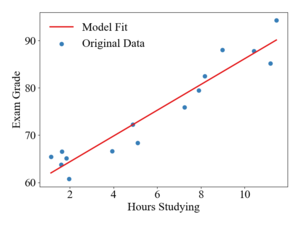
To illustrate how updates occur in the Adam algorithm, consider a linear, least-squares regression problem formulation. The table below shows a sample data-set of student exam grades and the number of hours spent studying for the exam. The goal of this example will be to generate a linear model to predict exam grades as a function of time spent studying.

Hours Studying	9.0	4.9	1.6	1.9	7.9	2.0	11.5	3.9	1.1	1.6	5.1	8.2	7.3	10.4	11.2
Exam Grad	88.0	72.3	66.5	65.1	79.5	60.8	94.3,	66.7	65.4	63.8	68.4	82.5	75.9	87.8	85.2

The hypothesized model function will be

$f_{\theta }(x)=\theta _{0}+\theta _{1}x.$

The cost function is defined as

$J({\theta })={\frac {1}{2}}\sum _{i}^{n}{\big (}f_{\theta }(x_{i})-y_{i}{\big )}^{2},$

Where the $1/2$ coefficient is used only to make the derivatives cleaner. The optimization problem can then be formulated as trying to find the values of $\theta$ that minimize the squared residuals of $f_{\theta }(x)$ and $y$.

$\mathrm {argmin} _{\theta }\quad {\frac {1}{n}}\sum _{i}^{n}{\big (}f_{\theta }(x_{i})-y_{i}{\big )}^{2}$

For simplicity, parameters will be updated after every data point i.e. a batch size of 1. For a single data point the derivatives of the cost function with respect to $\theta _{0}$ and $\theta _{1}$ are

${\frac {\partial J(\theta )}{\partial \theta _{0}}}={\big (}f_{\theta }(x)-y{\big )}$
${\frac {\partial J(\theta )}{\partial \theta _{1}}}={\big (}f_{\theta }(x)-y{\big )}x$

The initial values of ${\theta }$ will be set to [50, 1] and The learning rate, $\alpha$, is set to 0.1 and the suggested parameters for $\beta _{1}$, $\beta _{2}$, and $\epsilon$ are used. With the first data sample of $(x,y)=[8.98,88.01]$, the computed gradients are

${\frac {\partial J(\theta )}{\partial \theta _{0}}}={\big (}(50+1\cdot 9-88.01{\big )}=-29.0$
${\frac {\partial J(\theta )}{\partial \theta _{1}}}={\big (}(50+1\cdot 9-88.01{\big )}\cdot 9.0=-261$

With $m_{0}$ and $v_{0}$ being initialized to zero, the calculations of $m_{1}$ and $v_{1}$ are

$m_{1}=0.9\cdot 0+(1-0.9)\cdot {\begin{bmatrix}-29\\-261\end{bmatrix}}={\begin{bmatrix}-2.9\\-26.1\end{bmatrix}}$
$v_{1}=0.999\cdot 0+(1-0.999)\cdot {\begin{bmatrix}-29^{2}\\-261^{2}\end{bmatrix}}={\begin{bmatrix}0.84\\68.2\end{bmatrix}},$

The bias-corrected terms are computed as

${\hat {m}}_{1}={\begin{bmatrix}-2.9\\-26.1\end{bmatrix}}{\frac {1}{(1-0.9^{1})}}={\begin{bmatrix}-29.0\\-261.1\end{bmatrix}}$
${\hat {v}}_{1}={\begin{bmatrix}0.84\\68.2\end{bmatrix}}{\frac {1}{(1-0.999^{1})}}={\begin{bmatrix}851.5\\68168\end{bmatrix}}.$

Finally, the parameter update is

$\theta _{0}=50-0.1\cdot -29/({\sqrt {851.5}}+10^{-8})=50.1$
$\theta _{1}=1-0.1\cdot -261/({\sqrt {68168}}+10^{-8})=1.1$

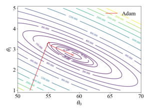
This procedure is repeated until the parameters have converged, giving $\theta$ values of $[58.98,2.72]$. The figures to the right show the trajectory of the Adam algorithm over a contour plot of the objective function and the resulting model fit. It should be noted that the stochastic gradient descent algorithm with a learning rate of 0.1 diverges and with a rate of 0.01, SGD oscillates around the global minimum due to the large magnitudes of the gradient in the $\theta _{1}$ direction.

Applications

Comparison of training a multilayer neural network on MNIST images for different gradient descent algorithms published in the original Adam paper (Kingma, 2015)¹.

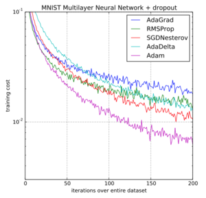
The Adam optimization algorithm has been widely used in machine learning applications to train model parameters. When used with backpropagation, the Adam algorithm has been shown to be a very robust and efficient method for training artificial neural networks and is capable of working well with a variety of structures and applications. In their original paper, the authors present three different training examples, logistic regression, multi-layer neural networks for classification of MNIST images, and a convolutional neural network (CNN). The training results from the original Adam paper showing the objective function cost vs. the iteration over the entire data set for the multi-layer neural network is shown to the right.

Variants of Adam

AdaMax

AdaMax¹ is a variant of the Adam algorithm proposed in the original Adam paper that uses an exponentially weighted infinity norm instead of the second-order moment estimate. The weighted infinity norm updated $u_{t}$, is computed as

$u_{t}=\max(\beta _{2}\cdot u_{t-1},|g_{t}|).$

The parameter update then becomes

$\theta _{t}=\theta _{t-1}-(\alpha /(1-\beta _{1}^{t}))\cdot m_{t}/u_{t}.$

Nadam

The Nadam algorithm⁵ was proposed in 2016 and incorporates the Nesterov Accelerate Gradient (NAG, a popular momentum like SGD variation, into the first-order moment term.

Conclusion

Adam is a variant of the gradient descent algorithm that has been widely adopted in the machine learning community. Adam can be seen as the combination of two other variants of gradient descent, SGD with momentum and RMSProp. Adam uses estimations of the first and second-order moments of the gradient to adapt the parameter update. These moment estimations are computed via moving averages,$m_{t}$ and$v_{t}$, of the gradient and the squared gradient respectfully. In a variety of neural network training applications, Adam has shown increased convergence and robustness over other gradient descent algorithms and is often recommended as the default optimizer for training ⁶.

References

1. Kingma, Diederik P., and Jimmy Lei Ba. Adam: A Method for Stochastic Optimization. 3rd International Conference on Learning Representations, ICLR 2015 - Conference Track Proceedings, 2015, pp. 1–15.
2. Ruder, Sebastian. An Overview of Gradient Descent Optimization Algorithms, 2016, pp. 1–14, http://arxiv.org/abs/1609.04747.
3. Tieleman, Tijmen, and Hinton, Geoffrey. Lecture 6.5-rmsprop: Divide the gradient by a running average of its recent magnitude, COURSERA: Neural Networks for Machine Learning, 2012.
4. Dozat, Timothy. Incorporating Nesterov Momentum into Adam. ICLR Workshop, no. 1, 2016, pp. 2013–16.
5. Nesterov, Yuri. A method of solving a convex programming problem with convergence rate O(1/k^2). In Soviet Mathematics Doklady, 1983, pp. 372-376.
6. "Neural Networks Part 3: Learning and Evaluation," CS231n: Convolutional Neural Networks for Visual Recognition, Stanford Unversity, 2020