Disjunctive inequalities
Introduction
Disjunctive inequalities are a form of disjunctive constraints that can be applied to linear programming. Disjunctive constraints are applied in all disjunctive programming, which just refers to the use of logical constraints, which include the “Or” and “And” statements. In order to solve a disjunctive, the constraints have to be converted into multiple integer programming (MIP) constraints, which is called disjunction. Disjunction involves the implementation of a binary variable to create a new set of constraints that can be solved easily. Two common methods for disjunction are the Big-M Reformulation and the Convex-Hull Reformulation.
Method
General
When given a set of inequalities, such as $ f_1(x)\ \le\ 0\ \And \ f_2(x)\ \le\ 0 $, the disjunctive form is given by: $ \begin{bmatrix} y \\ f_1(x)\ \le\ 0 \end{bmatrix} \lor \begin{bmatrix} -y \\ f_2(x)\ \le\ 0 \end{bmatrix} $. In order to turn the problem into a solvable MIP or MILP, logical constraints are created by using sufficiently large numbers, such as M1 and M2, and a binary variable y for each inequality. This is shown below by M1, M2, y1, and y1:
$ f_1(x)\ \le\ M_1\ast(1-y_1) $
$ f_2(x)\ \le\ M_2\ast(1-y_2) $
To set the binary variable to be mutually exclusive, the sum of the variables is set to 1 and the range is set to {0,1}.
$ y_1\ +y_2\ =\ 1 $
$ y_1\ ,\ y_2\epsilon\ {0,1}\ \ $
Big-M Reformulation

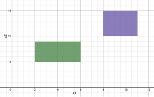
For the Big-M reformulation, a sufficiently large number, M, is used to nullify one set of constraints. This is accomplished by adding or subtracting the term “M*(1-y)” to the upper bound and lower bound constraints, respectively, with its respective binary variable. For example, given a solution space $ \begin{bmatrix} y \\ 2\le\ x_1\ \le6 \\ 5\le\ x_2\ \le9 \end{bmatrix} \lor \begin{bmatrix} -y \\ 8\le\ x_1\ \le11 \\ 10\le\ x_2\ \le15\ \end{bmatrix} $(shown graphically in Figure 1), to determine which of the solutions is optimal, the problem must be formulated such that one set of constraints is chosen. Using the Big-M Reformulation, the following MILP set would be obtained:
y Formulation
$ 2 - M*(1-y_1) \leq x1 \leq 6 + M*(1-y_1) $
$ 5 - M*(1-y_1) \leq x2 \leq 9 + M*(1-y_1) $
-y Formulation
$ 8 - M*(1-y_2) \leq x1 \leq 11 + M*(1-y_2) $
$ 10 - M*(1-y_2) \leq x2 \leq 15 + M*(1-y_2) $
Convex-Hull Reformulation
Similar to the Big-M reformulation, the convex-hull reformulation uses a binary variable, y, to constrain the set of inequalities. The first step in converting the problem into a solvable MILP is breaking all variables into a set of variables, such as (x1 → x11 + x12). By adding these addition variables, it is possible to isolate what set of parameters provide for the optimal solution of the problem. Then, similar to the Big-M reformulation, a sufficiently large variable, M, is used to nullify the non-optimal variable set, such as x11 and x12. For the problem show in Figure 1, the following variable constraints would be formulated:
y Formulation
$ 0 \leq x_{11} \leq M*y_1 $
$ 0 \leq x_{21} \leq M*y_1 $
-y Formulation
$ 0 \leq x_{12} \leq M*y_2 $
$ 0 \leq x_{22} \leq M*y_2 $
Formulation of the numerical constraints would then be implemented: y Formulation
$ 2\ast y_1\le\ x_{11}\ \le6\ast y_1 $
$ 5\ast y1\le\ x_{21}\ \le9\ast y1 $
-y Formulation
$ 8\ast y_2\le\ x_{12}\ \le11\ast y_2 $
$ 10\ast y_2\le\ x_{22}\ \le15\ast y_2 $
With the Convex-Hull transformation, the additional constraints confine the problem, such that a tighter (convex) solution space is examined compared to Big-M Formulation.
Examples
Applications
Conclusion
References
- ↑ L.A. Wolsey, Integer Programming, pp 130 - 133. Wiley, 1998.
Authors: Daniel Ladron, Grant Logan, Matthew Dinh, Derek Moore (CBE/SysEn 6800, Fall 2021)