Bayesian Optimization

Author : Deepa Korani

Steward : Fenqgi You

Introduction

In black-box optimization the goal is to solve the problem min_{x∈Ω} $f(x)$, where $f$ is a computationally expensive black-box function and the domain Ω is commonly a hyper-rectangle. Due to the fact that evaluations are computationally expensive, the goal is to reduce the number of evaluations of $f$ to a few hundred. In the black-box setting, no additional information is known about $f$. Hence, there is no observation of first- or second-order information when evaluating $f$ . This is commonly referred to as derivative-free optimization.

Black-box optimization problems of this form appear everywhere. Most machine learning (ML) models have hyperparameters that require tuning via black-box (i.e., derivative-free) optimization.These black-box optimization problems can be solved using Bayesian Optimization (BO) methods. BO rely on a surrogate model for the objective function that provides a measure of uncertainty.

Moreover many non Machine Learning based methods also benefit from the use of BO. For example, material discovery, manufacturing design are also effective uses of BO.

Methodology

Bayesian Optimization Algorithm has two main components :

Probabilistic Model

The other word for the probabilistic model is called as the surrogate function or the posterior distribution . The posterior captures the updated belief about the unknown objective function. A better interpretation of this is to estimate the objective the function with a surrogate function. Common Surrogate function used to model is the Gaussian Process (GP). Other probabilistic models are Random Forests, and Tree Parzen Estimators .

Here in the Gaussian Process is described in detail:

Gaussian Process[GP]

Gaussian Process can be described as a collection of random variables, where any finite number of the function $f$ are jointly normally distributed. It is defined by a mean function $m[x]$ and a covariance function $k[x,x']$ that returns similarity among two points. The Gaussian process models the objective function as: $f[x]\sim GP[m[x],k[x,x']]$ which states that:

$E[f[x]]-m[x]$

Given observations $f=[f[x_{1}],f[x_{2}],\dotsc ,f[x_{t}]]$ at $t$ points, the objective is to make prediction about the function value at a new point $x^{\star }$. This new function value $f^{\star }=f[x^{\star }]$ is jointly normally distributed with the observations $f$ so that:

$\mathbf {Pr} {\begin{pmatrix}{\begin{bmatrix}f\\f*\end{bmatrix}}\end{pmatrix}}=\mathbf {Norm} {\begin{bmatrix}0,&{\begin{bmatrix}K[X,X]&K[X,x^{\star }]\\K[x^{\star },X]&K[x^{\star },x^{\star }]\end{bmatrix}}\end{bmatrix}}$

where $K[X,X]$ is a $t\times t$ matrix where element $(i,j)$ is given by $k[xi,xj],K[X,x^{\star }]$ is a $t\times 1$ vector where element $i$ is given by $k[x_{i},x^{\star }]$ and so on.

Since the function values in equation above are jointly normal, the conditional distribution $Pr(f^{\star }\vert f)$ must also be normal, and thereby the standard formula for the mean and variance of this conditional distribution becomes:

$Pr(f^{\star }\vert f)=Norm[\mu [x^{\star }],\sigma ^{2}[x^{\star }]]$

where:

$\mu [x^{\star }]$ = $K[x^{\star },X]$ $[K[X,X]]^{-1}$ $f$

$\sigma ^{2}[x^{\star }]$ =$K[x^{\star },x^{\star }]$ − $K[x^{\star },X]$ $[K[X,X]]^{-1}$ $K[X,x^{\star }]$

Using this formula, the distribution of the function at any new point $x^{\star }$ can be estimated.The best estimate of the function value is given by the mean $\mu [x]$ , and the uncertainty is given by the variance $\sigma ^{2}[x]$.

Acquisition Function

The second component of Bayesian Optimization is the Acquistion Function.The role of the acquisition function is to guide the search for the optimum. Typically, acquisition functions are defined such that high acquisition corresponds to potentially high values of the objective function, whether because the prediction is high, the uncertainty is great, or both. Maximizing the acquisition function is used to select the next point at which to evaluate the function. Hence the main goal is to sample $f$ at $\arg \max$ $x_{u(x|D)}$ , where $u$ is the generic symbol for an acquisition function.

A good acquisition function should trade off exploration and exploitation. Two typically used acquisition functions are the Probability of Improvement (PI) and the Expected Improvement (EI) . In PI, the probability that sampling a given data-point, $x$, improves over the current best observation is maximized. One problem with the approach taken in PI is that it will, by its nature, prefer a point with a small but certain improvement over one which offers a far greater improvement, but at a slightly higher risk. In order to combat this effect, EI proposes maximizing the expected improvement over the current best known point.EI has been shown to have strong theoretical guarantees and empirical effectiveness , and is often used as the acquistion function as a baseline. The formulations of common acquisition functions, Upper Bound Confidence, Probability of Improvement and Expected Improvement are defined below:

Upper Bound Confidence

This acquisition function is defined as:

$UCB[x^{\star }]$ = $\mu [x^{\star }]$ + $\beta ^{1/2}$ $\sigma [x*]$

Probability of Improvement

This acquisition function computes the likelihood that the function at x∗ will return a result higher than the current maximum $f[{\hat {x}}]$ . For each point x∗, the goal is to integrate the part of the associated normal distribution that is above the current maximum (figure 4b) such that:

$PI[x^{\star }]$ = $\int _{f[x]}^{\infty }$ $Norm_{f[x^{\star }]}$ $[\mu [x^{\star }]],\sigma [x^{\star }]]$ $df[x^{\star }]$

Expected Improvement

The expected Improvement can be modelled as:

$EI[x^{\star }]$ = $\int _{f[{\hat {x}}]}^{\infty }$ $(f[x^{\star }]-f[{\hat {x}}])$ $Norm_{f[{\hat {x}}]}$ $[\mu [x^{\star }],\sigma [x^{\star }]]$ $df[x^{\star }]$

Algorithm

Here follows a longer example of mathematical-style pseudocode, for the Bayesian Optimization :

1: Algorithm' Bayesian Optimization ' is
2:    for t == 1,2,.....do  
3:         Find xt by optimizing the the acquisition function over the GP: xt = argmaxxu(x|D1:t-1)
4:         Sample the objective function yt = f(xt) + εt
5:         Augment the data D1:t = {D1:t-1,(xt,yt)} and update the GP
6:    end for

Applications

Bayesian Optimization has shown a wide variety of interest in areas of data science and Chemical Engineering, Material Science domain. Certain application include; robotics, environmental monitoring, combinatorial optimization, adaptive Monte Carlo, reinforcement learning. Some of the applications are described below in detail:

• A/B Testing - Though the idea of A/B testing dates back to the early days of advertising in the form of so-called focus groups, the advent of the internet and smartphones has given web and app developers a new forum for implementing these tests at unprecedented scales. By redirecting small fractions of user traffic to experimental designs of an ad, app, game, or website, the developers can utilize noisy feedback to optimize any observable metric with respect to the product’s configuration. In fact, depending on the particular phase of a product’s life, new subscriptions may be more valuable than revenue or user retention, or vice versa; the click-through rate might be the relevant objective to optimize for an ad, whereas for a game it may be some measure of user engagement. The crucial problem is how to optimally query these subsets of users in order to find the best product with high probability within a predetermined query budget, or how to redirect traffic sequentially in order to optimize a cumulative metric while incurring the least opportunity cost.
• Recommender Systems - Generally Recommender systems are used by online content providers to recommend products to their subscribers. Recommending the right product to subscribers is important in order to improvise the revenue in case for e-commerce sits, or consumption sites.
• Natural Language Processing and Text- Bayesian Optimization has been applied to improve text extraction.
• Environmental Monitoring and Sensor Networks - Sensor Networks allow monitoring important environment conditions; such as temperature, concentration of pollutants in the atmosphere, soil and ocean. These networks make noise measurements that are interpolated to produce a global model of interest. In some cases, these sensors are expensive to activate but one can answer important questions like what is the hottest or coldest spot in a building by activating a relatively small number of sensors. Bayesian optimization was used for this task and the similar one of finding the location of greatest highway traffic congestion
• Materials - Bayesian Optimization is applied to design experiments of previous experiments to suggest features of the new materials whose performance is evaluated by simulation. Final goal is to improvise the design while reducing the number of experimentation. Bayesian Optimization are used to predict compounds with low thermal conductivity , optimal melting temperature , elastic properties

Numerical Example

Here using the HyperOpt package ; a simple optimization problem will be solved: The example is broken down into four steps:

Problem Set Up

The minimization problem can be defined as:

$x^{\star }=\arg \min f(x)$

In this problem $f$ is a fixed objective function that is evaluated pointwise. The first assumption is that there is no access to the gradient of $f$. A second assumption is the evaluations of $f$ is noisy.

The problem is solved by using Bayesian Optimization, and defining the prior, a posterior to derive an acquisition function at each time step. In order to solve using BO, a sequence of points ${x_{n}}$ will be constructed that converge to $x^{\star }$.

Objective Function

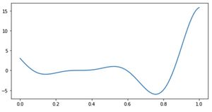
The objective function for this example is a simple function defined below. The objective function has both a local and a global minimum as seen in Figure 1. The global minimum is at $x^{\star }=0.75725$ $f(x)=(6x-2)^{2}$ $sin(12x-4)$ , $x\epsilon [0,1]$

Figure 1 : Objective Function : $f(x)=(6x-2)^{2}$ $sin(12x-4)$

Setting a Gaussian Process Prior

As described earlier, the Gaussian Process is most commonly used as the prior, for Bayesian Optimization.

In the example: Given inputs $X$ and the corresponding noise observations $y$, the model takes the form:

$f\sim MultivariateNormal(0,k(X,X))$, $y\sim f+\epsilon$

The domain is the value of $x$ over which the function is evaluated. Hence a uniform distribution is utilized in this case over the space of function defined.

In the equation below, $\epsilon$ is i.i.d Gaussian noise and $k(X,X)$ is a covariance matrix whose entries are given by $k(x,x^{\prime })$ for each pair of inputs $(x,x^{\prime })$

Define Acquistion Function

For this problem, the acquisition function used is the Lower Confidence Bound acquisition function due to its simplicity and easy interpretability.

The Lower Confidence Bound acquisition function is defined as :

$\alpha (x)=\mu (x)-\kappa \sigma (x)$

Here in $\mu (x)$ and $\sigma (x)$ are the mean and square root variance of the posterior at point $x$

Results and Running the Optimization

Once the acquisition function and Prior is defined; the acquisition function is used to derive the next query point as follows : $x_{n+1}=\arg \min \alpha (x)$ and then Evaluate $f(x_{n+1})$ and update the posterior, until convergence.

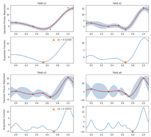
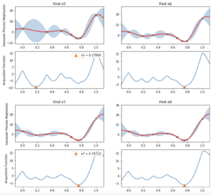
Results for the first 8 iterations for the Gaussian Process Regression and Acquistion functions are shown in Figure 2 and Figure 3. As one of the assumptions stated earlier was that the observation contain noise, it is impossible to converge to the ground truth solution.However, as seen in Figure 2 an 3; with a limited budget of 8 evaluations; BO has converged close to the global minimum at $x^{\star }=0.75725$

Figure 2: GPR and Acquistion Function plots for first four time steps

Figure 4: GPR and Acquistion Function for next four iterations

Bayesian Optimization Packages

Here are a list of packages in Python, Java, C++that utelize Bayesian Optimization

Table - Packages Utilizing Bayesian Optimization

Package	License	URL	Language	Model
SMAC	Academic	http://www.cs.ubc.ca/labs/beta/Projects/SMAC	Java	Random Forest
Hyperopt	BSD	https://github.com/hyperopt/hyperopt	Python	Tree Parzen Estimator
Spearmint	Academic	https://github.com/HIPS/Spearmint	Python	Gaussian Process
Bayesopt	GPL	https://github.com/rmcantin/bayesopt	C++	Gaussian Process
PyBO	BSD	https://github.com/mwhoffman/pybo	Python	Gaussian Process
MOE	Apache 2.0	https://github.com/Yelp/MOE	Python/ C++	Gaussian Process

Conclusion

In conclusion; Bayesian Optimization primarily is utilized when Blackbox functions are expensive to evaluate and are noisy, and can be implemented easily in Python. Bayesian optimization uses a surrogate function to estimate the objective through sampling. These surrogates, Gaussian Process, are represented as probability distributions which can be updated in light of new information. The Acquisition functions, Upper Bound Confidence, Probability of Improvement, Expected Improvement, then are used to evaluate the probability of exploring a certain point in space will yield a good return. Lastly Bayesian optimization is often extended to complex problems including and not limited to hyperparameter tuning of machine learning models .

References

- ↑ R. Turner, D. Eriksson, M. Mccourt, and I. Guyon, “Bayesian Optimization is Superior to Random Search for Machine Learning Hyperparameter Tuning : arXiv : 2104 . 10201v2 [ cs . LG ] 31 Aug 2021,” 2020.
- ↑ J.Snoek,H.Larochelle,andR.P.Adams. PracticalBayesianoptimizationofmachinelearning algorithms. In Advances in Neural Information Processing Systems 25, pages 2960–2968, 2012.
- ↑ D. Eep, “F EW -S HOT B AYESIAN O PTIMIZATION K ERNEL S URROGATES,” pp. 1–15, 2021
- ↑ E. Brochu, V. M. Cora, and N. De Freitas, “arXiv : 1012 . 2599v1 [ cs . LG ] 12 Dec 2010 A Tutorial on Bayesian Optimization of Expensive Cost Functions , with Application to Active User Modeling and Hierarchical Reinforcement Learning,” 2010.
- ↑ F. Hutter, H. H. Hoos, and K. Leyton-brown, “Sequential Model-Based Optimization for General Algorithm Configuration ( extended version ).”
- ↑ J. Bergstra, “Algorithms for Hyper-Parameter Optimization,” pp. 1–9.
- ↑ D. Jasrasaria and E. O. Pyzer-knapp, “Dynamic Control of Explore / Exploit Trade-Off In Bayesian Optimization,” no. July, 2018.
- ↑ B. J. Snoek, H. Larochelle, and R. P. Adams, “PRACTICAL BAYESIAN OPTIMIZATION OF MACHINE LEARNING,” pp. 1–12.
- ↑ K. Swersky et al., “Taking the Human Out of the Loop : A Review of Bayesian Optimization Taking the Human Out of the Loop : A Review of Bayesian Optimization,” 2016, doi: 10.1109/JPROC.2015.2494218.
- ↑ Z. Wang and L. Jin, “Bayesian Multi-Scale Optimistic Optimization,” vol. 33, 2014.
- ↑ N. Srinivas, A. Krause, and M. Seeger, “Gaussian Process Optimization in the Bandit Setting : No Regret and Experimental Design,” 2010.
- ↑ A. Seko, H. Hayashi, K. Tsuda, L. Chaput, and I. Tanaka, “Prediction of Low-Thermal-Conductivity Compounds with First-Principles Anharmonic Lattice-Dynamics Calculations and Bayesian Optimization,” doi: 10.1103/PhysRevLett.115.205901.
- ↑ A. Seko, T. Maekawa, K. Tsuda, and I. Tanaka, “to melting temperatures of single and binary component solids,” pp. 1–10, 2018.
- ↑ D. Xue, P. V Balachandran, J. Hogden, J. Theiler, D. Xue, and T. Lookman, “properties by adaptive design,” pp. 1–9, 2016, doi: 10.1038/ncomms11241.
- ↑ Bergstra, J., Yamins, D., Cox, D. D. (2013) Making a Science of Model Search: Hyperparameter Optimization in Hundreds of Dimensions for Vision Architectures. To appear in Proc. of the 30th International Conference on Machine Learning (ICML 2013).
- ↑ Wu, J.; Hao, X. C.; Xiong, Z. L.; Lei, H. Hyperparameter Optimization for Machine Learning Models Based on Bayesian Optimization. J. Electron. Sci. Technol. 2019, 17 (1), 26–40. https://doi.org/10.11989/JEST.1674-862X.80904120.