FTRL algorithm

Author: Tsz Ki Peter Wei (tmw86), Nhi Nguyen (npn25), Colin Erb (cte24) (ChemE 6800 Fall 2024)

Stewards: Nathan Preuss, Wei-Han Chen, Tianqi Xiao, Guoqing Hu

Introduction

The FTRL (Follow the Regularized Leader) family of learning algorithms is a core set of learning methods used in online learning. As a type of FTL (Follow the Leader) algorithm, they select a weight function at each timestep that minimizes the loss of all previously observed data. To reduce computational complexity, implementations of the FTRL algorithm generally utilize a linearized loss function, while a regularizer ensures solution stability by limiting changes to the weight vector. The algorithm was originally introduced in 2008 by J.D. Abernethy, E. Hazan, and A. Rakhlin, with the key idea of “analysis through the dual” The use of linear losses in FTRL started in 2009 with the publishing of a paper by Y. Nesterov, although the idea is claimed to have originated in 2001-2002 but was deemed unimportant . It is currently popular due to its asymptotically optimal regret and, in certain implementations, model sparsity in contrast to generic FTL algorithms, which have the dependency to overfit given a lack of regularization while minimizing total loss with the dimensionality available. A version of the algorithm using L1 and L2 regularizers was popularized by Google for ad-click advertising, specifically to predict ad click-through rates for sponsored search advertising.

Algorithm Discussion

General Algorithm Description:

The FTRL algorithm is designed to minimize the objective function shown below.

$w_{t+1}=\arg \min \left(l_{1:t}(w)+R(w)\right)$

This minimization problem finds the weight vector minimizing the function $f(w)=l_{1:t}(w)+R(w)$, where $l_{1:t}(w)$ represents the cumulative loss of all previous observations, and $R(w)$ is a regularization term. Solving this objective, however, is extremely computationally expensive, as the loss must be expanded and recomputed for all past data points whenever new data is introduced.  

To address this, most implementations of the algorithm approximate the loss using a linearized loss function, leveraging the gradient of the original loss to reduce computational complexity. Unlike other machine learning algorithms that iteratively step along this gradient upon each update step, FTRL minimizes an optimization problem upon each update step, where instead the regularization places a limit on the step size.

In order to evaluate the effectiveness of the model, the regret bound provides a strong metric for how well the model converges, by illustrating how similar previous predictions of the weight vector align to the optimal prediction generated using more data.  FTRL has a regret bound of the following form:

${\text{Regret}}(u)\leq R(u)+\sum _{t=1}^{T}\left(l_{t}(w_{t})-l_{t}(w_{t+1})\right)$ 

This indicates that the total regret is constrained by two factors, those being the regularization and cumulative loss from updating the weight vector with new data.  This expression is derived from the below relation.

$\sum _{t=0}^{T}\left(f_{t}(w_{t})-f_{t}(u)\right)\leq \sum _{t=0}^{T}\left(f_{t}(w_{t})-f_{t}(w_{t+1})\right)$

This lemma holds true, as at best $f_{t}(w_{t+1})$ is equal to $f_{t}(u)$ for all run times. In practice, the presence of the regularization term prevents $f_{t}(w_{t})$ from matching the optimal solution, but it helps minimize regret in more noisy environments, where the decision variable between steps varies significantly without it.

Common Implementations:

Linear Loss FTRL

One of the simplest forms of the FTRL algorithm utilizes a linearized loss function, reducing the cost of recomputing all past losses, and an L₂ regularization term to stabilize the solution. As such, the weight update is defined as follows :

$w_{t+1}=\arg \min _{w\in \mathbb {R} ^{n}}\left(g_{1:t}\cdot w+{\frac {1}{2\eta }}\|w\|_{2}^{2}\right)$Minimizing this expression involves setting the gradient with respect to weight vector to 0:

$\nabla _{w}\left(g_{1:t}\cdot w+{\frac {1}{2\eta }}\|w\|_{2}^{2}\right)=g_{1:t}+{\frac {1}{\eta }}w=0\implies w=-\eta g_{1:t}$

In the update step, the gradient of the loss function, $g_{1:t}$ can be approximated as $g_{1:t}=-\eta \left(g_{t}+{\frac {-w_{t}}{\eta }}\right)$, based on the solution to the previous iteration producing a solution for w. Utilizing this, the weight vector update for each new data point becomes $w_{t+1}=w_{t}-\eta g_{t}$.

This is the same formulation as that of gradient descent, making this a special case of the FTRL algorithm , and shows an important parallel between the formulations and how their processing of data compares, despite the different problem formulations.

Model Pseudo-code:

Initialize parameters:

s = 0

z = 0

w=0

for each iteration t= 1 ... T:

1. (x_t, y_t): Receive a new data point.
2. (${\hat {y}}_{t}=\mathbf {w} ^{\top }\mathbf {x} _{t}$): Compute the predicted value.
3. ($g_{1:t}=-\eta \left(g_{t}+{\frac {\mathbf {w} _{t}}{\eta }}\right)$): Compute the accumulating gradient of the loss function L.
4. ($\mathbf {w} _{t+1}=-\eta g_{1:t}$):Update the weight vector.

FTRL-Proximal algorithm

Some kinds of regularization terms, such as that used in ad-click advertising by Google, combine both L1 and L2 loss to produce solutions that are both stable and sparse, similarly to other online gradient descent algorithms such as Objective Constraint Online Gradient Descent (OC-OGD). An instance of the FTRL algorithm using both L1 and L2 regularization terms is shown below.  

$w=\arg \min \left(g_{t}^{\top }w+\sum _{s=1}^{t}{\frac {1}{2\eta _{s}}}\|w-w_{s}\|^{2}+t\lambda \|w\|_{1}\right)$

This version of the FTRL algorithm is particularly adept at introducing sparsity, given the t copies of the L1 regularization term introduced for each time step in the online update process . It promotes model stability as the dataset size grows via the second term in the model, which decreases each weight’s update size proportionally to its update history. The solution for the weight vector update is shown below, with i representing each dimension.

$w_{t+1,i}={\begin{cases}-\eta _{t}\left(z_{t,i}-{\text{sign}}(z_{t,i})\lambda _{1}\right),&{\text{if }}|z_{t,i}|\leq \lambda _{1}\\0&{\text{otherwise}}\end{cases}}$

$z_{t}=g_{1:t-1}-\sum _{s=1}^{t-1}\sigma _{s}w_{s}+g_{t}+\left({\frac {1}{\eta _{t}}}-{\frac {1}{\eta _{t-1}}}\right)w_{t}$.

Typically, the z value’s historical data would be saved, thus making the update step for z_t as follows:

$z_{t}=z_{t-1}+g_{t}+\left({\frac {1}{\eta _{t}}}-{\frac {1}{\eta _{t-1}}}\right)w_{t}$

The learning rate is set dynamically using the following relation, where α and β are hyper-parameters set ahead of time to maximize performance:

$\eta _{t,i}={\frac {\alpha }{\beta +{\sqrt {\sum _{s=1}^{t}g_{s,i}^{2}}}}}$

There are a few major consequences of this algorithm. The consideration of the L1 regularization and L2 regularization through stabilization encouraging sparse solutions where weights less than lambda are pulled to 0, and exceedingly large gradients across previous iterations are updated less, as to encourage more unstable dimensions to stabilize and allow stable dimensions room to explore. As such, this model balances stability and sparsity to form a highly versatile model.

Model Pseudocode:

Initialize parameters:

s = 0

z = 0

w=0

for each iteration t= 1 ... T:

1. (x_t, y_t): Receive a new data point.
2. (${\hat {y}}_{t}=\mathbf {w} ^{\top }\mathbf {x} _{t}$): Compute the predicted value.
3. ($g_{t,i}={\frac {\partial L({\hat {y}}_{t},y_{t})}{\partial \mathbf {w} }}$): Compute the gradient of the loss function L with respect to w.
4. ($\mathbf {s_{i}} =\mathbf {s_{i}} +(g_{i})^{2}$): Update the accumulated squared gradients.
5. ($\eta _{i}={\frac {\alpha }{{\sqrt {s_{i}}}+\beta }}$): Update the learning rate for each feature i.
6. ($z_{t,i}=z_{t-1,i}+g_{t,i}+\left({\frac {1}{\eta _{t}}}-{\frac {1}{\eta _{t-1}}}\right)w_{t,i}$): Update the z-values for each feature i.
7. ($w_{t+1,i}={\begin{cases}-\eta _{t,i}\left(z_{t,i}-{\text{sign}}(z_{t,i})\lambda _{1}\right)&{\text{if }}|z_{t,i}|>\lambda _{1}\\0&{\text{otherwise}}\end{cases}}$): Update the weight vector

Numerical Examples

Example 1: Linear Loss with Quadratic Regularization

Problem Setup:

• Decision variable: $w\in \mathbb {R}$,
• Loss functions: $f_{t}(w)=a_{t}w$, where $a_{t}$ are coefficients provided by the environment. In the case of a linear loss function, $a_{t}$ determines the slope or gradient of the loss function $f_{t}(w)$,
• Regularization: $R(w)={\frac {\lambda }{2}}w^{2}$, where $\lambda$ is a hyperparameter that determines the update rate.

FTRL Update Rule: The update rule is: $w_{t+1}=\arg \min _{w}\left(\sum _{i=1}^{t}a_{i}w+{\frac {\lambda }{2}}w^{2}\right).$

To minimize, take the derivative and set it to zero: ${\frac {\partial }{\partial w}}\left(\sum _{i=1}^{t}a_{i}w+{\frac {\lambda }{2}}w^{2}\right)=\sum _{i=1}^{t}a_{i}+\lambda w=0.$

Rearranging gives: $w_{t+1}=-{\frac {\sum _{i=1}^{t}a_{i}}{\lambda }}.$

Step-by-Step Calculation: Let the gradient of the loss functions be $a_{1}=-1$, $a_{2}=1.75$, $a_{3}=-1.95$, initialize $w_{0}=0$, and choose $\lambda =3$.

• Iteration 1:

$w_{1}=-{\frac {a_{1}}{\lambda }}=-{\frac {-1}{3}}=0.33.$

• Iteration 2:

$w_{2}=-{\frac {a_{1}+a_{2}}{\lambda }}=-{\frac {(-1)+1.75}{3}}=-0.25.$

• Iteration 3:

  

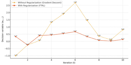
  Fig 1. Stabilizing effects of FTRL for linear loss function.
  Without regularization (blue), updates fluctuate significantly. With regularization (orange), updates stabilize over tim

$w_{3}=-{\frac {a_{1}+a_{2}+a_{3}}{\lambda }}=-{\frac {(-1)+1.75+(-1.95)}{3}}=0.4.$

Observation: The updates for $w$ gradually converge rather than overshooting or oscillating, thanks to regularization reducing large shifts with the term $\lambda$ in the update rule. Decision variables calculated with and without the regularization term in the update rule (i.e. setting $\lambda =1$) are compared for 10 iterations to demonstrate this stabilizing effect.

• Without Regularization: Updates ($w_{t}$) exhibit significant fluctuations as they respond solely to the cumulative gradients $\sum _{i=1}^{t}a_{i}$.
• With Regularization: Updates are smoother, as the regularization term $\lambda$ reduces the influence of cumulative gradients, stabilizing the updates over time.

Example 2: Quadratic Loss with Quadratic Regularization

Problem Setup:

• Quadratic loss function: $f_{t}(w)={\frac {1}{2}}(w-b_{t})^{2}$, where $b_{t}$ is the target set by the adversary,
• Regularization: $R(w)={\frac {\lambda }{2}}w^{2}$.

FTRL Update Rule: The update rule becomes: $w_{t+1}=\arg \min _{w}\left(\sum _{i=1}^{t}{\frac {1}{2}}(w-b_{i})^{2}+{\frac {\lambda }{2}}w^{2}\right).$

Simplifying: $w_{t+1}={\frac {\sum _{i=1}^{t}b_{i}}{t+\lambda }}.$

Step-by-Step Calculation: Let coefficients $b_{1}=1$, $b_{2}=2$, $b_{3}=3$, initialize $w_{0}=0$, and choose $\lambda =2$.

• Iteration 1:

$w_{1}={\frac {b_{1}}{1+\lambda }}={\frac {1}{1+2}}=0.33.$

• Iteration 2:

$w_{2}={\frac {b_{1}+b_{2}}{2+\lambda }}={\frac {1+2}{2+2}}=0.75.$

• Iteration 3:

  

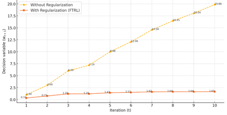
  Fig 2. Stabilizing effects of FTRL for quadratic loss function.
  Without regularization (blue), updates grow unbounded. With regularization (orange), updates converge gradually.

$w_{3}={\frac {b_{1}+b_{2}+b_{3}}{3+\lambda }}={\frac {1+2+3}{3+2}}=1.2.$

Observation: The denominator $t+\lambda$ ensures that updates become smaller over time, stabilizing the solution as more data is observed. Decision variables calculated with and without the regularization term are compared for 10 iterations to demonstrate this stabilizing effect in Figure 2.

• Without Regularization: Linear and unbounded growth. Updates ($w_{t}$) grow rapidly as they are driven entirely by the cumulative target values $\sum _{i=1}^{t}b_{i}$, leading to unbounded growth over time.
• With Regularization: Gradual convergence with stabilized updates. The denominator $t+\lambda$ dampens the influence of cumulative targets, stabilizing the updates.

Application

The FTRL algorithm is a powerful framework for online learning problems due to its ability to handle large datasets and adapt to new data in real-time. It has been applied in finance, healthcare, and electrical engineering. In finance, the FTRL algorithm has been used in online advertising, e-commerce recommendations, and fraud detection . In healthcare, the FTRL algorithm has been used for the analysis of patient data . In electrical engineering, the FTRL algorithm has been used to optimize the performance of electrical power systems . Specific case studies of the FTRL algorithm in each field are shown below.

Finance

The first application that the FTRL algorithm was used for was online advertising by Google . In this case study, the FTRL algorithm was used to predict ad click-through rates (CTR) for sponsored search advertising at Google . They were able to demonstrate the FTRL algorithm’s ability to both predict accurately and also be sparse compared to other online learning algorithms . Additional case studies in the finance sector have been explored such as online portfolio optimization . In this case study, the authors were able to build off the original FTRL algorithm to come up with a new algorithm called VB-FTRL that can maximize a trader’s return on their portfolio while having reduced runtime compared to the best-performing algorithm (Universal Portfolios) .  

Healthcare

In healthcare, the FTRL algorithm was used in a case study to classify thyroid nodules for Thyroid cancer diagnosis . In this case study, the authors proposed a novel FTRL-Deep Neural Network technique to precisely classify thyroid nodules into benign or malignant. The algorithm would analyze ultrasound images of the thyroid nodules and then determine whether or not the patient has thyroid cancer or not . They were able to show that their FTRL-Deep Neural Network algorithm had superior accuracy compared to other algorithms such as the Hybrid Feature Cropping Network and Multi-Channel Convolutional Neural Network .

Electrical Engineering

Recently, FTRL has been applied to electrical power systems. A recent case study used FTRL to optimize the output of a solar panel system to offset the effect of non-uniform irradiance . They developed this algorithm to control a system of switches that would determine the optimal configuration of the solar panel array when non-uniform irradiance is detected to maximize the power output from the solar panel . In an earlier case study, researchers were able to use an FTRL algorithm to predict when low voltages would occur in a power distribution system, allowing for better system management .

Softwares and Platforms that Utilize the FTRL Algorithm

Software tools such as H2O Driverless AI and Keras can utilize the FTRL algorithm for various machine-learning applications . In addition, platforms such as Google Ads utilize the FTRL algorithm . These are just a few examples of softwares and platforms where the FTRL algorithm is used. As machine-learning becomes more and more widespread in different applications, the usage of the FTRL algorithm is expected to increase.

Conclusion

The FTRL algorithm is most useful in online learning, where large amounts of data need to be processed in real time to enable accurate predictions. Currently, the FTRL algorithm is used on platforms such as Google Ads and included in software tools such as Keras and H2O driverless AI. In recent years, other areas of application that involve online learning, such as healthcare and power systems, have been explored for the FTRL algorithm.

The algorithm works through a minimization of a linearized loss function considering all historical data and at least one regularization term every time a new point is added. This minimization operation is reasonably space and time-efficient due to linearization, and due to flexibility in how the weight vector is regularized, very versatile. The simplest implementation of the algorithm is equivalent to gradient descent, while more complex versions of the algorithm are able to effectively stabilize the weight vector as the dataset grows and maintain sparsity in its updates through the inclusion of an L1 norm.

From the numerical examples, it is evident that regularization plays a pivotal role in ensuring convergence. For linear loss functions, FTRL mitigates oscillatory behavior by reducing the influence of cumulative gradients. For quadratic loss functions, regularization stabilizes updates over time, resulting in gradual convergence and bounded growth. These properties underline FTRL's adaptability in noisy environments and its capacity to produce reliable predictions.

Looking ahead, potential areas for improvement include enhancing computational efficiency for more complex loss functions and exploring hybrid regularization schemes that combine the strengths of L1, L2, and other techniques. Additionally, further advancements in applying FTRL to evolving fields such as autonomous systems, environmental modeling, and personalized medicine could broaden its impact.

References

Stewards: Nathan Preuss, Wei-Han Chen, Tianqi Xiao, Guoqing Hu

References

- ↑ 1.0 1.1 [1] bremen79, “Follow-The-Regularized-Leader I: Regret Equality,” Parameter-free Learning and Optimization Algorithms. Accessed: Dec. 03, 2024. [Online]. Available: https://parameterfree.com/2019/10/08/follow-the-regularized-leader-i-regret-equality
- ↑ 2.0 2.1 2.2 2.3 2.4 2.5 2.6 2.7 H. B. McMahan et al., “Ad click prediction: a view from the trenches,” in Proceedings of the 19th ACM SIGKDD international conference on Knowledge discovery and data mining, Chicago Illinois USA: ACM, Aug. 2013, pp. 1222–1230. doi: 10.1145/2487575.2488200.
- ↑ 3.0 3.1 3.2 [1] B. McMahan, “Follow-the-regularized-leader,” CSE599s, https://courses.cs.washington.edu/courses/cse599s/14sp/scribes/lecture3/lecture3.pdf (accessed Dec. 14, 2024).
- ↑ 4.0 4.1 [1] B. McMahan, “The FTRL algorithm with strongly convex Regularizers,” cse599s, https://courses.cs.washington.edu/courses/cse599s/12sp/scribes/Lecture8.pdf (accessed Dec. 14, 2024).
- ↑ 5.0 5.1 J. O. Schneppat, “Follow The Regularized Leader (FTRL),” Schneppat AI. Accessed: Nov. 30, 2024. [Online]. Available: https://schneppat.com/follow-the-regularized-leader_ftrl.html
- ↑ Z. Ye, F. Chen, and Y. Jiang, “Analysis and Privacy Protection of Healthcare Data Using Digital Signature,” in Proceedings of the 2024 3rd International Conference on Cryptography, Network Security and Communication Technology, Harbin China: ACM, Jan. 2024, pp. 171–176. doi: 10.1145/3673277.3673307.
- ↑ 7.0 7.1 7.2 X. Gao et al., “Followed The Regularized Leader (FTRL) prediction model based photovoltaic array reconfiguration for mitigation of mismatch losses in partial shading condition,” IET Renew. Power Gener., vol. 16, no. 1, pp. 159–176, 2022, doi: 10.1049/rpg2.12275.
- ↑ 8.0 8.1 C. Gao, Z. Ding, S. Yan, and H. Mai, “Low Voltage Prediction Based on Spark and Ftrl,” in Proceedings of the Advances in Materials, Machinery, Electrical Engineering (AMMEE 2017), Tianjin City, China: Atlantis Press, 2017. doi: 10.2991/ammee-17.2017.34.
- ↑ 9.0 9.1 R. Jézéquel, D. M. Ostrovskii, and P. Gaillard, “Efficient and Near-Optimal Online Portfolio Selection,” Sep. 28, 2022, arXiv: arXiv:2209.13932. doi: 10.48550/arXiv.2209.13932.
- ↑ 10.0 10.1 10.2 A. Beyyala, R. Priya, S. R. Choudari, and R. Bhavani, “Classification of Thyroid Nodules Using Follow the Regularized Leader Optimization Based Deep Neural Networks. | EBSCOhost.” Accessed: Nov. 30, 2024. [Online]. Available: https://openurl.ebsco.com/contentitem/doi:10.18280%2Fria.370315?sid=ebsco:plink:crawler&id=ebsco:doi:10.18280%2Fria.370315
- ↑ “Supported Algorithms — Using Driverless AI 1.11.0 documentation.” Accessed: Nov. 30, 2024. [Online]. Available: https://docs.h2o.ai/driverless-ai/1-10-lts/docs/userguide/supported-algorithms.html
- ↑ K. Team, “Keras documentation: Ftrl.” Accessed: Nov. 30, 2024. [Online]. Available: https://keras.io/api/optimizers/ftrl/