Optimization in game theory
Authors: Jego Fonseca, Caroline Grala, Max Johnson, Lauren Ribordy, Dean Schifilliti (SysEn 5800 Fall 2021)
Introduction
Game Theory (GT) is a branch of mathematics that analyzes and predicts trends in a number of different game scenarios with a varying number of players. The application of GT can be found in a multitude of disciplines, including economics, biology, political science, computer systems, and philosophy. [1]
Emile Borel has been credited with being the first mathematician to suggest a formal theory of games in 1921, but the popularity of GT became more apparent in 1944 when John von Neumann and Oskar Morgenstern published “Theory of Games and Economic Behavior”. In the 1950s and 1960s, GT application was expanded to war, politics, philosophy, and political and social sciences. [1]
In general, games are broken down into two main categories: noncooperative and cooperative. Within these two categories, many different game types exist. Noncooperative games are defined as games where “each participant acts independently, without collaborating with the others, and chooses their strategy for improving their own benefit,” whereas cooperative games are defined as games where “a set of players seek to form cooperative groups to improve their performance in a competitive game, and to enable players to succeed in reaching objectives that they may not accomplish independently”. [1]
Optimal choices and their relative influence on the game can be analyzed through the mathematical methods in GT. However, the number of possible combinations increases exponentially with the number of players, so the optimal solution may not always be a computationally realistic possibility. This article aims to discuss the theory and methodology, provide numerical examples, and discuss the applications of GT. [1]
Theory, methodology, and/or algorithmic discussions
Theory

The Nash equilibrium is a fundamental concept in game theory. It is most widely used in predicting the outcome of a strategic interaction in the social sciences. A game consists of: a set of players, a set of actions available to each player, and a payoff function for each player. The payoff function is a player’s preference of the action profiles. A “pure-strategy Nash equilibrium” is an action profile with the property that no single player can obtain a higher payoff by deviating from this profile. [3]
The classic game Prisoners’ Dilemma is widely used to demonstrate the Nash equilibrium. In this decision game, if one player stays silent while the other talks, that player will get 10 years in prison. If they both talk, they both get 8 years. If neither talk, they both will get 2 years. The Nash equilibrium for this game is each player talking and getting 8 years. While both players staying silent is the optimal solution, neither of the players have incentive from deviating to this profile because the player who remains silent is worse off. [2]
Methodology
Nash equilibrium is commonly used as an example to describe a non-cooperative game involving two or more people. Mixed Integer Linear Programming (MILP) is an optimization method that aims to either maximize or minimize a linear objective function given at least one constraint. In addition, some of the variables in a MILP problem are discrete while others are continuous. Nash equilibrium can be found through mixed-integer linear programming optimization. It can also be found using other optimization methodologies, such as the one created by Tsaknakis and Spirakis. Their method takes the maximum deviation of a player’s payoff from the best payoff that could be achieved by the other players based on their strategy of choice. [4]
Linear programming (LP) is another method used in optimization to describe a problem that has an objective function, constraints, and variables that are both linear and continuous. It can be used to determine an optimal strategy for simple games like rock-paper-scissors or more complex ones like poker. [5] The goal is similar to an MILP problem in that it quantifies decision consequences in order to achieve a specific outcome. [6] For the rock-paper-scissors game where there are two players involved, one player’s set of options are defined as a, where a = {1, 2, and 3} and the other as b, where b = {1, 2, and 3}. Each player can decide from one of three options, i.e. rock, represented by the number 1 and so forth. Their choice results in either a win, loss, or draw with the payoff represented by 1, -1, or 0, respectively. Depending on the established amount of times that the game is played, a matrix can be generated to model the outcome and size from the set of decisions made by both players.
Algorithm

The common algorithm associated with computing a Nash Equilibrium is the Lemke-Howson algorithm. This algorithm utilizes iterated pivoting much like the simplex algorithm used in linear programming. A notable difference between the two algorithms is that unlike the simplex algorithm, the Lemke-Howson algorithm cannot be run in polynomial time. The Lemke-Howson algorithm can be considered a brute force algorithm in which we utilize a possible solution as a guess and continue to adjust it through each iteration until we have arrived at the Nash equilibrium. [4]
The tableau method is a pivoting process that can be used to find the Nash equilibrium using the Lemke-Howson algorithm. The first step is preprocessing, the goal here is to limit the options of the game by iterating to maintain the dominating strategies. This reduces the problem complexity and thus the work required to solve it. The initialization of the tableau is the next step. One tableau is needed for each player in the game. Now with a constructed tableau we can begin pivoting. The primary aspect here are the entry and exit variables. The exit variable is the entry variable to the next pivot until the complementarity conditions are met. [4]
The algorithm flow consists of four primary steps. Preprocessing is the first step, which consists of reducing the solution space by ruling out strictly dominated strategies. Tableaux Initilizations involve creating a tableaux for all involved parties in the game. With all tableauxs created the next step is pivoting. By chosing the basis variable to enter and exit on, multiple iterations of pivoting can be performed to fund the output which is the final step of the process.
Numerical Example
Overview
A town has two competitors for taxi services—Beru and Fylt. Consumers choose between the two companies based on their prices and availability, i.e. the cost of a ride based on distance and the wait time for a ride.
Beru has more availability, but has historically higher prices. Fylt is a newcomer looking to challenge Beru. Fylt is trying to decide how to develop its brand and where it stands to make most profit: capturing the market for people who take long and expensive but inconvenient rides, such as going to the airport, or for people who take short and inexpensive but convenient rides, such as going to a grocery store.
Problem Statement
Fylt’s data analysis department has analyzed sales data and created the following strategic form price matrices for both long and short distance rides:
| Beru | |||
|---|---|---|---|
| Long distance, high ($) | Long distance, low ($) | ||
| Fylt | Long distance, high ($) | F: 90, B: 160 | F: 50, B: 250 |
| Long distance, low ($) | F: 200, B: 150 | F: 100, B: 150 | |
| Beru | |||
|---|---|---|---|
| Short distance, high ($) | Short distance, low ($) | ||
| Fylt | Short distance, high ($) | F: 50, B: 60 | F: 10, B: 30 |
| Short distance, low ($) | F: 70, B: 20 | F: 50, B: 30 | |
As a member of the Fylt finance department, it is your job to calculate the dominant strategies for both Beru and Fylt based on the price matrices from the data analysis department.
You are expected to answer the following specific questions:
- Is there a dominant strategy for Beru and/or Fylt? If so, what is it?
- What is the Nash equilibrium, if it exists?
- How should Fylt invest to outcompete Beru—in doing more short or long distance trips?
Solution
- To calculate the dominant strategies, create 4 diagrams.
- The number of diagrams is determined by the numbers of competitors (2) multiplies by the number of scenarios to consider (the number of price matrices). This problem is thus represented by 4 diagrams in total.
- There should be 2 diagrams for the long distance case and 2 for the short distance case, and respectively a Beru and Fylt each. The final diagrams should be Long-Fylt, Long-Beru, Short-Fylt, Short-Beru.
- Populate the diagrams with data from the price matrices.
- For the example of Long-Fylt, fill out the values that Beru gains based on whether Fylt chooses the high or low option. The Long Distance Price Matrix contains all values needed for this example.
- For the example of Short-Beru, fill out the values that Fylt gains based on whether Beru chooses the high or low option. The Short Distance Price Matrix contains all values needed for this example.
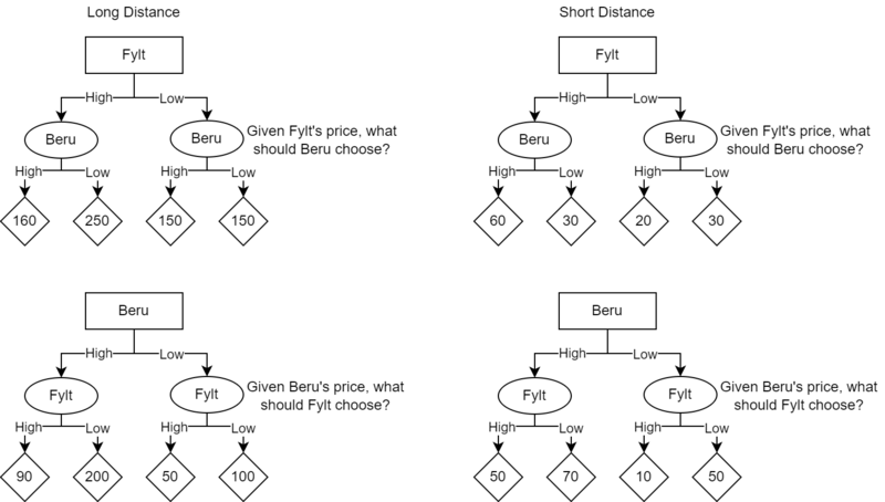
A diagram to assist in determining the optimal dominant strategies for Beru and Fylt. Diagram created by the authors using draw.io
- Find the best strategies at each node for Beru and Fylt.
- For each diagram's terminal node, circle the optimal choice for Fylt or Beru. Because we are maximizing gains in this example, the highest value is the optimal value
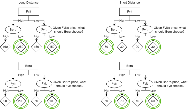
Demonstration of how to evaluate the strategies for Fylt and Beru based on their cost matrices. Diagram created by the authors using draw.io
- For each diagram's terminal node, circle the optimal choice for Fylt or Beru. Because we are maximizing gains in this example, the highest value is the optimal value
- Determine the dominant strategies for Beru and Fylt.
- There exists a dominant strategy when no matter what the competitor chooses to do (i.e. price high or low), the company will always make the same choice.
- In the Long-Fylt example, if Fylt prices high, Beru should price low; and if Fylt prices low, Beru should still price low. Beru thus has a dominant strategy for pricing low.
- In the Short-Fylt example, if Fylt prices high, Beru should price high; and if Fylt prices low, Beru should price low. Because Beru's strategy is dependent on Fylt's choice, it does not have a dominant strategy.
- Calculate the Nash equilibrium, if it exists.
- The Nash equilibrium is the optimal strategy that the two competitors settle on. A Nash equilibrium is not always guaranteed (i.e. for a trivial case where all options produce the exact same benefits and are indistinguishable from one another).
- Determine the Nash equilibrium by referencing the diagrams created above. For instance, for long distances, we see that both Beru and Fylt always pick the low option for their dominant strategies. For short distances, we notice that while Fylt does not have a dominant strategy, Beru does: going low. Because Beru always goes low, then the optimal choice for Fylt is also going low.


Answering the Original Questions
Is there a dominant strategy for Beru and/or Fylt? If so, what is it?
When the distance is far, the dominant strategies for both Beru and Fylt are to set low prices.
When the distance is short, Beru does not have a dominant strategy because its optimal price depends on whether Fylt chooses to price low or high. If Fylt prices low, Beru should go low; but if Fylt prices high, Beru should go high. Fylt has a dominant strategy for short distances: low prices.
What is the Nash equilibrium, if it exists?
Based on the data, the Nash equilibrium for short distances and long distances is for Beru and Fylt to both set low prices. So for far trips, Beru will make 150, and Fylt 100. For short trips, Beru will make 30 and Fylt will make 50.
How should Fylt invest to outcompete Beru—in doing more short or long distance trips?
Fylt should invest in scaling up its short distance trips, as this is the only area in which it has a profit advantage over Beru.
Applications
The application of GT can be found across a multitude of disciplines, but the general framework of GT allows players to compare the outcomes of different decisions. A list of popular applications for GT will be discussed, and these game examples can be altered and applied to a wide range of scenarios.
Game Examples
Stag Hunt
This game balances safety and social cooperation. Two hunters go for a hunt, and each must choose to hunt a stag or a hare, without knowing which the other chooses. In order for the hunters to take down a stag, both must hunt the stag. Each may hunt a hare individually, but the payoff from the hare is less than that of the stag. The goal is to maximize payoff. [1]
The Battle of Sexes
This game falls into the category of coordination games and is based around the decisions for what two individuals will do on a given night. For instance, a girlfriend and boyfriend prefer to go to the opera and a football game, respectively. They do not decide on where they are going before leaving for the day and do not communicate with each other throughout the day. They prefer the place that they chose, but they would prefer to go to the same place. The goal is to maximize happiness. [1]
The Prisoner’s Dilemma
Two criminals are arrested, imprisoned, and isolated from each other. Without enough evidence to accuse either criminal of a crime, there are three possible outcomes: both reveal evidence and both stay in prison for 4 years, one reveals evidence and one stays silent so the one that reveals is set free while the one that stays silent serves 5 years, and if both prisoners stay silent then both will only remain in prison for 2 years. The goal is to minimize prison time. [1]
Extensions of GT
Evolutionary Game Theory
GT was developed on human interaction, but the theory was applied in biology to model how animals behave when competing for a resource. Rather than using logic, the players, or animals, instead are motivated by reproductive success. In Evolutionary Game Theory, the success is based on the frequency of success against competing strategies. In the end, successful strategies will be used more frequently and be the final victor. [1]
Behavioral Game Theory
While computers may try to optimize utility and use perfect logic, humans have been found to not always use logic or maximize utility. Instead, Behavioral Game Theory attempts to model and predict human choices in games, rather than advise the optimal solution. Experimental data is leveraged to show trends and account for external factors, such as emotions, bounded rationality, cultural influences, and reputation among others on the decisions that humans make in games. [1]
Mechanism Design
Mechanism design introduces a reverse approach to GT in that the objective is known while the rules and mechanisms are unknown. The game must be designed such that players are incentivized to behave as the designer intended. As an example, a Vickrey auction style is an example of auctioning where the good goes to the highest bidder at the price of the second-highest bid. This form of game incentivizes players to be honest in their evaluation of the good. [1]
Conclusion
This article summarized GT, a branch of mathematics that analyzes and predicts trends in a number of different game scenarios with a varying number of players. The Nash Equilibrium is a fundamental concept in GT and is commonly used as an example to describe a non-cooperative game involving two or more people. Both MILP and LP are useful programming styles to solve various problems within GT. The common algorithm associated with computing a Nash Equilibrium is the Lemke-Howson algorithm. [4] A numerical example based on taxi services was detailed and the steps for completing it were outlined. Finally, a few examples of common games that utilize GT and a few extensions of GT were discussed. GT has existed since 1921, is still applied today, and will continue to be useful to individuals across all disciplines.
References
- ↑ 1.00 1.01 1.02 1.03 1.04 1.05 1.06 1.07 1.08 1.09 Burguillo, Juan C. “Game Theory.” Self-Organizing Coalitions for Managing Complexity, 2017, pp. 101–135., https://doi.org/10.1007/978-3-319-69898-4_7.
- ↑ 2.0 2.1 S. Woodcock, “The legacy of John Nash and his equilibrium theory,” The Conversation, 21-Oct-2019. [Online]. Available: https://theconversation.com/the-legacy-of-john-nash-and-his-equilibrium-theory-42343. [Accessed: 10-Dec-2021].
- ↑ R. A. McCain, Game theory and public policy. Cheltenham: Edward Elgar, 2010.
- ↑ 4.0 4.1 4.2 4.3 D. Pritchard, “Game Theory F07,” pp. 1–7.
- ↑ N. Dotzenrod and M. Kweon, “Matrix game (LP for game theory),” Northwestern University Open Text Book on Process Optimization. [Online]. Available: https://optimization.mccormick.northwestern.edu/index.php/Matrix_game_(LP_for_game_theory). [Accessed: 10-Dec-2021].
- ↑ F. You, “6800-LP F21,” in SYSEN 5800 Lecture.