Line search methods
Authors: Lihe Cao, Zhengyi Sui, Jiaqi Zhang, Yuqing Yan, and Yuhui Gu (6800 Fall 2021).
Introduction
Line search method is an iterative approach to find a local minimum of a multidimensional nonlinear function using the function's gradients. It computes a search direction and then finds an acceptable step length that satisfies certain standard conditions. [1] Line search method can be categorized into exact and inexact methods. The exact method, as in the name, aims to find the exact minimizer at each iteration; while the inexact method computes step lengths to satisfy conditions including Wolfe and Goldstein conditions. Line search and trust-region methods are two fundamental strategies for locating the new iterate given the current point. With the ability to solve the unconstrained optimization problem, line search is widely used in many cases including machine learning, game theory and other fields.
Generic Line Search Method
Basic Algorithm
- Pick the starting point $ x_0 $
- Repeat the following steps until $ f_k:=f(x_k) $ coverges to a local minimum :
- Choose a descent direction $ p_k $ starting at $ x_k $, defined as: $ \nabla f_{k}^\top p_{k}<0 $ for $ \nabla f_k \not =0 $
- Find a step length $ \alpha_k>0 $ so that $ f(x_k+\alpha_kp_k)<f_k $
- Set $ x_{k+1}=x_k+\alpha_k p_k $
Search Direction for Line Search
The direction of the line search should be chosen to make $ f $ decrease moving from point $ x_k $ to $ x_{k+1} $, and it is usually related to the gradient $ \nabla f_k $. The most obvious direction is the $ - \nabla f_k $ because it is the one to make $ f $ decreases most rapidly. This claim can be verified by Taylor's theorem:
$ f(x_k+\alpha)=f(x_k)+\alpha p^\top\nabla f_k+\frac{1}{2}\alpha^2p^\top f(x_k+tp)p $, where $ t\in (0, \alpha) $.
The rate of change in $ f $ along the direction $ p $ at $ x_k $ is the coefficient of $ \alpha $. Therefore, the unit direction $ p $ of most rapid decrease is the solution to
$ \min\ p^\top\nabla f_k $
$ \text{s.t.}\ \ ||p||=1 $.
$ p=\frac{-\nabla f_k}{||\nabla f_k||} $ is the solution and this direction is orthogonal to the contours of the function. In the following sections, this will be used as the default direction of the line search.
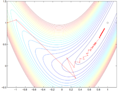
However, the steepest descent direction is not the most efficient, as the steepest descent method does not pass the Rosenbrock test (see Figure 1). [2] Carefully designed descent directions deviating from the steepest direction can be used in practice to produce faster convergence. [3]
Step Length
The step length is a non-negative value such that $ f(x_k+\alpha_k p_k)<f(x_k) $. When choosing the step length $ \alpha_k $, there is a trade off between giving a substantial reduction of $ f $ and not spending too much time finding the solution. If $ \alpha_k $ is too large, then the step will overshoot, while if the step length is too small, it is time consuming to find the convergent point. An exact line search and inexact line search are needed to find the value of $ \alpha $ and more detail about these approaches will be introduced in the next section.
Convergence
For a line search algorithm to be reliable, it should be globally convergent, that is the gradient norms, $ ||\nabla f(x_{k})|| $, should converge to zero with each iteration, i.e., $ \lim_{k\to\infty} ||\nabla f(x_{k})|| = 0 $.
It can be shown from Zoutendijk's theorem [1] that if the line search algorithm satisfies (weak) Wolfe's conditions (similar results also hold for strong Wolfe and Goldstein conditions) and has a search direction that makes an angle with the steepest descent direction that is bounded away from 90°, the algorithm is globally convergent.
Zoutendijk's theorem states that, given an iteration where $ p_k $ is the descent direction and $ \alpha_k $ is the step length that satisfies (weak) Wolfe conditions, if the objective $ f $ is bounded below on $ \mathbb{R}^{n} $ and is continuously differentiable in an open set $ \mathcal{N} $ containing the level set $ \mathcal{L}:=\{x\ |\ f(x)\leq f(x_0)\} $, where $ x_0 $ is the starting point of the iteration, and the gradient $ \nabla f $ is Lipschitz continuous on $ \mathcal{N} $, then
$ \sum_{k=0}^{\infty}\cos^{2}\theta_{k}||\nabla f_{k}||^2 < \infty $,
where $ \theta_{k} $ is the angle between $ p_k $ and the steepest descent direction $ -\nabla f(x_{k}) $.
The Zoutendijk condition above implies that
$ \lim_{k\to\infty}\cos^{2}\theta_{k}||\nabla f_{k}||^2=0 $,
by the n-th term divergence test. Hence, if the algorithm chooses a search direction that is bounded away from 90° relative to the gradient, i.e., given $ \epsilon>0 $,
$ \cos\theta_{k}\geq\epsilon>0,\ \forall k $,
it follows that
$ \lim_{k\to\infty}||\nabla f_{k}||=0 $.
However, the Zoutendijk condition doesn't guarantee convergence to a local minimum but only stationary points. Hence, additional conditions on the search direction is necessary, such as finding a direction of negative curvature whenever possible, to avoid converging to a nonminimizing stationary point.
Exact Search
Steepest Descent Method
Given the intuition that the negative gradient $ - \nabla f_k $ can be an effective search direction, steepest descent follows the idea and establishes a systematic method for minimizing the objective function. Setting $ - \nabla f_k $ as the direction, steepest descent computes the step-length $ \alpha_k $ by minimizing a single-variable objective function. More specifically, the steps of Steepest Descent Method are as follows:
Steepest Descent Algorithm
Set a starting point $ x_0 $
Set a convergence criterium $ \epsilon>0 $
Set $ k = 0 $
Set the maximum iteration $ N $
While $ k \le N $:
- $ \nabla f(x_k) = \left.\frac{\partial f(x)}{\partial x}\right\vert_{x=x_k} $
- If $ \nabla f(x_k)\le \epsilon $:
- Break
- End if
$ \alpha_k=\underset{\alpha}{\arg\min} f(x_k-\alpha \nabla f(x_k)) $
$ x_{k+1}=x_k-\alpha_k \nabla f(x_k) $
$ k = k + 1 $
End while
Return $ x_{k} $, $ f(x_{k}) $

One advantage of the steepest descent method is the convergency. For a steepest descent method, it converges to a local minimum from any starting point. [4]
Theorem: Global Convergence of Steepest Descent
Let the gradient of $ f \in C^1 $ be uniformly Lipschitz continuous on $ \mathbb{R}^{n} $. Then, for the iterates with steepest-descent search directions, one of the following situations occurs:
- $ \nabla f(x_k) = 0 $ for some finite $ k $
- $ \lim_{k \to \infty} f(x_k) = -\infty $
- $ \lim_{k \to \infty} \nabla f(x_k) = 0 $
However, steepest descent has disadvantages in that the convergence is always slow and numerically may be not convergent (see Figure 1.)
Steepest descent method is a special case of gradient descent in that the step-length is analytically defined. However, step-lengths cannot always be computed analytically; in this case, inexact methods can be used to optimize $ \alpha $ at each iteration.
Inexact Search
While minimizing an objective function using numeric methods, in each iteration, the updated objective is $ \phi(\alpha) = f(x_k+\alpha p_k) $, which is a function of $ \alpha $ after fixing the search direction. The goal is to minimize this objective with respect to $ \alpha $. However, if one wants to solve for the exact minimum in each iteration, it could be computationally expensive and the algorithm will be time-consuming. Therefore, in practice, it is easier solve the subproblem
$ \underset{\alpha}{min} \quad \phi(\alpha) = f(x_k + \alpha p_k) $
numerically and find a reasonable step length $ \alpha $ instead, which will decrease the objective function. That is, $ \alpha $ satisfies $ f(x_k + \alpha p_k) \leq f(x_k) $. However, convergence to the function's minimum cannot be guaranteed, so Wolfe or Goldstein conditions need to be applied when searching for an acceptable step length. [1]
Wolfe Conditions
This condition is proposed by Phillip Wolfe in 1969. [5] It provide an efficient way of choosing a step length that decreases the objective function sufficiently. It consists of two conditions: Armijo (sufficient decrease) condition and the curvature condition.

Armijo (Sufficient Decrease) Condition
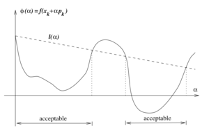
$ f(x_k + \alpha p_k) \leq f(x_k) + c_1 \alpha_{k} p^\top_k \nabla{f(x_k)} $,
where $ c_1\in(0,1) $ and is often chosen to be of a small order of magnitude around $ 10^{-3} $. This condition ensures the computed step length can sufficiently decrease the objective function $ f(x_k) $. Only using this condition, however, it cannot be guaranteed that $ x_k $ will converge in a reasonable number of iterations, since Armijo condition is always satisfied with step length being small enough. Therefore, the second condition below needs to be paired with the sufficient decrease condition to keep $ \alpha_k $ from being too short.
Curvature Condition

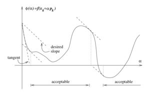
$ \nabla{f(x_k + \alpha p_k)}^\top p_k \geq c_2 \nabla{f(x_k)}^\top p_k $,
where $ c_2\in(c_1,1) $ is much greater than $ c_1 $ and is typically on the order of $ 0.1 $. This condition ensures a sufficient increase of the gradient.
This left hand side of the curvature condition is simply the derivative of $ \phi(\alpha) $, thus ensuring $ \alpha_k $ to be in the vicinity of a stationary point of $ \phi(\alpha) $.
Strong Wolfe Curvature Condition
The (weak) Wolfe conditions can result in an $ \alpha $ value that is not close to the minimizer of $ \phi(\alpha) $. The (weak) Wolfe conditions can be modified by using the following condition called Strong Wolfe condition, which writes the curvature condition in absolute values:
$ |p_k \nabla{f(x_k + \alpha p_k)| \leq c_2 |p^\top_k f(x_k)}| $.
The strong Wolfe curvature condition restricts the slope of $ \phi(\alpha) $ from getting too positive, hence excluding points far away from the stationary point of $ \phi $.

Goldstein Conditions
Another condition to find an appropriate step length is called Goldstein conditions:
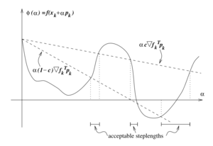
$ f(x_k) + (1-c) \alpha_k \nabla{f^\top_k} p_k \leq f(x_k + \alpha p_k) \leq f(x_k) + c \alpha_k \nabla{f^\top_k} p_k $
where $ 0 \leq c \leq 1/2 $. The Goldstein condition is quite similar with the Wolfe condition in that, its second inequality ensures that the step length $ \alpha $ will decrease the objective function sufficiently and its first inequality keep $ \alpha $ from being too short. In comparison with Wolfe condition, one disadvantage of Goldstein condition is that the first inequality of the condition might exclude all minimizers of $ \phi $ function. However, usually it is not a fatal problem as long as the objective decreases in the direction of convergence. As a short conclusion, the Goldstein and Wolfe conditions have quite similar convergence theories. Compared to the Wolfe conditions, the Goldstein conditions are often used in Newton-type methods but are not well-suited for quasi-Newton methods that maintain a positive definite Hessian approximation.
Backtracking Line Search
The backtracking method is often used to find the appropriate step length and terminate line search based. The backtracking method starts with a relatively large initial step length (e.g., 1 for Newton method), then iteratively shrinking it by a contraction factor until the Armijo (sufficient decrease) condition is satisfied. The advantage of this approach is that the curvature condition needs not be considered, and the step length found at each line search iterate is ensured to be short enough to satisfy sufficient decrease but large enough to still allow the algorithm to make reasonable progress towards convergence.
The backtracking algorithm involves control parameters $ \rho\in(0,1) $ and $ c\in(0,1) $, and it is roughly as follows:
- Choose $ \alpha_0>0, \rho\in(0,1), c\in(0,1) $
- Set $ \alpha\leftarrow\alpha_0 $
- While $ f(x_{k}+\alpha p_{k}) > f(x_{k})+c\alpha\nabla f_{k}^{\top}p_{k} $
- $ \alpha\leftarrow\rho\alpha $
- End while
- Return $ \alpha_k=\alpha $
Numeric Example
As an example, we can use line search method to solve the following unconstrained optimization problem:
$ \min_{x_1,x_2}\ f(x)=x_1-x_2+2x_1x_2+2x_1^2+x_2^2 $.
First iteration:
We have $ \nabla f(x)=\begin{bmatrix} 1+2x_2+4x_1\\ -1+2x_1+2x_2 \end{bmatrix} $.
Starting from $ x_0=\begin{bmatrix} 0\\0 \end{bmatrix} $ gives $ -\nabla f(x_0)=\begin{bmatrix}-1\\1\end{bmatrix} $.
We then have $ f(x_0-\alpha\nabla f(x_0))=f(-\alpha,\alpha)=\alpha^2-2\alpha $.
Taking partial derivative of the above equation with respect to $ \alpha $ and set it to zero to find the minimizer $ \alpha_0=1 $.
Therefore, $ x_1=\begin{bmatrix}0\\0\end{bmatrix} +\alpha_0 \begin{bmatrix}-1\\1\end{bmatrix} =\begin{bmatrix}-1\\1\end{bmatrix} $.
Second iteration:
Given $ x_1=\begin{bmatrix}-1\\1\end{bmatrix} $, we have $ -\nabla f(x_1)=\begin{bmatrix}1\\1\end{bmatrix} $.
Then from $ \min_\alpha f(x_1-\alpha\nabla f(x_1))=5\alpha^2-2\alpha-1 $, finding the minimizer $ \alpha_1=0.2 $.
Hence, $ x_2=\begin{bmatrix}-1\\1\end{bmatrix} +\alpha_1\begin{bmatrix}1\\1\end{bmatrix}=\begin{bmatrix}-0.8\\1.2\end{bmatrix} $.
Third iteration:
Given $ x_2=\begin{bmatrix}-0.8\\1.2\end{bmatrix} $, we have have $ -\nabla f(x_2)=\begin{bmatrix}-0.2\\0.2\end{bmatrix} $.
Then from $ \min_\alpha f(x_2-\alpha\nabla f(x_2))=0.04\alpha^2-0.08\alpha-1.2 $, finding the minimizer $ \alpha_2=1 $.
Hence, $ x_3=\begin{bmatrix}-0.8\\1.2\end{bmatrix} +\alpha_2\begin{bmatrix}-0.2\\0.2\end{bmatrix}=\begin{bmatrix}-1\\1.4\end{bmatrix} $.
Fourth iteration:
Given $ x_3=\begin{bmatrix}-1\\1.4\end{bmatrix} $, we have have $ -\nabla f(x_3)=\begin{bmatrix}0.2\\0.2\end{bmatrix} $.
Then from $ \min_\alpha f(x_3-\alpha\nabla f(x_3))=0.2\alpha^2-0.08\alpha-1.24 $, finding the minimizer $ \alpha_3=0.2 $.
Hence, $ x_4=\begin{bmatrix}-1\\1.4\end{bmatrix} +\alpha_3\begin{bmatrix}0.2\\0.2\end{bmatrix}=\begin{bmatrix}-0.96\\1.44\end{bmatrix} $.
Fifth iteration:
Given $ x_4=\begin{bmatrix}-0.96\\1.44\end{bmatrix} $, we have have $ -\nabla f(x_4)=\begin{bmatrix}-0.04\\0.04\end{bmatrix} $.
Then from $ \min_\alpha f(x_4-\alpha\nabla f(x_4))=0.0016 \alpha^2-0.0032 \alpha-1.248 $, finding the minimizer $ \alpha_4=1 $.
Hence, $ x_5=\begin{bmatrix}-0.96\\1.44\end{bmatrix} +\alpha_4\begin{bmatrix}-0.04\\0.04\end{bmatrix}=\begin{bmatrix}-1\\1.48\end{bmatrix} $.
Termination:
At this point, we find $ \nabla f(x_5)=\begin{bmatrix}-0.04\\-0.04\end{bmatrix} $.
Check to see if the convergence is sufficient by evaluating $ ||\nabla f(x_5)|| $:
$ || \nabla f(x_5)||=\sqrt{(-0.04)^2+(-0.04)^2}=0.0565 $.
Since $ 0.0565 $ is relatively small and is close enough to zero, the line search is complete.
The derived optimal solution is $ x^*=\begin{bmatrix}-1\\1.48\end{bmatrix} $, and the optimal objective value is found to be $ -1.25 $.
Applications
A common application of line search method is in minimizing the loss function in training machine learning models. For example, when training a classification model with logistic regression, gradient descent algorithm (GD), which is a classic method of line search, can be used to minimize the logistic loss and compute the coefficients by iteration till the loss function reaches converges to a local minimum. [6] An alternative of gradient descent in machine learning domain is stochastic gradient descent (SGD). The difference is on computation expense that instead of using all training set to compute the descent, SGD simply sample one data point to compute the descent. The application of SGD reduces the computation costs greatly in large dataset compared to gradient descent.
Line search methods are also used in solving nonlinear least squares problems, [7] [8] in adaptive filtering in process control, [9] in relaxation method with which to solve generalized Nash equilibrium problems, [10] in production planning involving non-linear fitness functions, [11] and more.
Conclusion
Line Search is a useful strategy to solve unconstrained optimization problems. The success of the line search algorithm depends on careful consideration of the choice of both the direction $ p_k $ and the step size $ \alpha_k $.This page has introduced the basic algorithm firstly, and then includes the exact search and inexact search. The exact search contains the steepest descent, and the inexact search covers the Wolfe and Goldstein conditions, backtracking, and Zoutendijk's theorem. More approaches to solve unconstrained optimization problems can be found in trust-region methods, conjugate gradient methods, Newton's method and Quasi-Newton method.
Reference
- ↑ 1.0 1.1 1.2 1.3 1.4 1.5 J. Nocedal and S. Wright, Numerical Optimization, Springer Science, 1999, p. 30-44.
- ↑ "Rosenbrock Function," Cornell University.
- ↑ R. Fletcher and M. Powell, "A Rapidly Convergent Descent Method for Minimization," The Computer Journal, vol. 6, no. 2, pp. 163–168, 1963.
- ↑ 4.0 4.1 R. Hauser, "Line Search Methods for Unconstrained Optimization," Oxford University Computing Laboratory, 2007.
- ↑ P. Wolfe, "Convergence Conditions for Ascent Methods," SIAM Review, vol. 11, no. 2, pp. 226–235, 1969.
- ↑ A. A. Tokuç, "Gradient Descent Equation in Logistic Regression."
- ↑ M. Al-Baali and R. Fletcher, "An Efficient Line Search for Nonlinear Least Squares," Journal of Optimization Theory and Applications, vol. 48, no. 3, pp. 359-377, 1986.
- ↑ P. Lindström and P. Å. Wedin, "A New Linesearch Algorithm for Nonlinear Least Squares Problems," Mathematical Programming, vol. 29, no. 3, pp. 268-296, 1984.
- ↑ C. E. Davila, "Line Search Algorithms for Adaptive Filtering," IEEE Transactions on Signal Processing, vol. 41, no. 7, pp. 2490-2494, 1993.
- ↑ A. von Heusinger and C. Kanzow, "Relaxation Methods for Generalized Nash Equilibrium Problems with Inexact Line Search," Journal of Optimization Theory and Applications, vol. 143, pp. 159–183, 2009.
- ↑ P. Vasant and N. Barsoum, "Hybrid Genetic Algorithms and Line Search Method for Industrial Production Planning with Non-linear Fitness Function," Engineering Applications of Artificial Intelligence, vol. 22, no. 4-5, pp. 767-777, 2009.