Portfolio optimization: Difference between revisions

Revision as of 23:03, 28 November 2021

Authors: Ainsely Li (fl366), Kevin Pan (kp428), Qizeng Sun (qs95), Hanshen Li (hl2436), Eric Luo (yl2429) Fall 2021

Introduction

Portfolio optimization is a way to minimize risks to maximize net gains in a portfolio. Apply probability statistics, linear algebra, optimization and other methods to redistribute the investment portfolio under the established target returns and risk limits to achieve the goal of reducing risks or obtaining higher benefits under the same risk conditions.

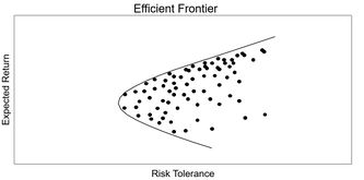
Risk is a major factor in choosing stocks in a portfolio. In order to mitigate these risks, investors typically use an efficient frontier graph as shown in figure 1.

The x- axis represents the standard deviation of the data, which is also known as the risk tolerance. On the y- axis is the expected percent return. The points near the solid line are optimal, which is also known as the frontier line. Any points that fall below the curve are considered to be nonoptimal. This is due to the fact that with the same risk tolerance there are better expected returns. This method has its limitations as it relies on past data.

Theory

The portfolio optimization mainly assumes two directions. The first is to assume that an investor has a fixed amount of investment in his hand, and requires to find one that has the smallest investment risk under certain relevant constraints of known investment projects. The other direction is to find a portfolio with the greatest return on investment under the same assumptions.

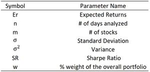
The mitigation of risk can be characterized as follows. Let A be a matrix mxn of the daily returns, where m is the number of stocks and n is the number of days that are being analyzed.

Er represents the expected returns of the stock which is the average of the individual column of M. σ is the standard deviation of the individual the data set of an individual stock, where σ $^{2}$ is the variance.

$X=A-Er$

X represents the daily return subtracted by the expected returns of each respective stock. The variance and covariance table is a vital tool as it allows the user to estimate volatility of the overall portfolio.

$\Sigma =(X^{T}*X)/(n-1)$

This table will span the size of the number of stocks chosen mxm.

$E(rp)=w*Er$

E(rp) is the expected return of the portfolio. w is the percent of the initial capital being allocated into each stock.

$\sigma _{p}=\surd (w*\Sigma *w^{T})$

σ $_{p}$ represents the standard deviation of the portfolio.

$SR_{p}=E(r_{p})/\sigma _{p})$

SR is the sharpe ratio. The sharpe ratio is a risk to return ratio that allows the investor to identify if the investment is worth the risk.

Methodology

Portfolio optimization could be solved and analyzed by Linear Programming and statistics. Cut the relevant information and conditions in the portfolio optimization, as well as the final requirements into the relevant variables, constraints and linear functions of the linear programming problem.

When figuring out the maximum return under the fixed risks investment projects:


Function	Max $\Sigma$ ri*Xi
Factor: Xi	The amount of investment project i should invest
Coefficient: ri	The risk of investment project i
Constants	The limit requirements

Constraints:

The constraints of portfolio optimization are various, include[4]:


Monetary value constraints	Turnover constraint
Long- only constraint	Maximum weight constraints
Asset trade constraints	Risk fraction constraints
Number of Assets Held Constraint	Number of Assets trade Constraint
Trade Universe Constraint	Threshold Constraints
Forced Trade Constraints	Linear Constraints
Count Constraints	Tracking Error Constraints
Volatility constraints	Expected return constraints
Distance constraints	Sum of largest weights constraints
Cost constraint	Number of closing positions constraint
Quadratic constraints	Round Lot constraints

In one portfolio optimization analysis, several types of constraints will be selected to formulate the final return. The difference of constraints depends on the differences in investment projects, and related policy requirements, etc.

Numerical Example

Example 1:

The example above is converted into the following table:

@@ Line 7: / Line 7: @@
 The x- axis represents the standard deviation of the data, which is also known as the risk tolerance. On the y- axis is the expected percent return. The points near the solid line are optimal, which is also known as the frontier line. Any points that fall below the curve are considered to be nonoptimal. This is due to the fact that with the same risk tolerance there are better expected returns. This method has its limitations as it relies on past data.
 [[File:Figure 1- Efficient Frontier Graph.jpg|thumb|333x333px|Figure 1: Efficient Frontier Graph]]
@@ Line 19: / Line 20: @@
 The mitigation of risk can be characterized as follows. Let '''A''' be a matrix mxn of the daily returns, where m is the number of stocks and n is the number of days that are being analyzed.
 '''Er''' represents the expected returns of the stock which is the average of the individual column of M. '''σ''' is the standard deviation of the individual the data set of an individual stock, where '''σ<math>^2</math>''' is the variance.
 <math>X = A - Er</math>
@@ Line 31: / Line 31: @@
 This table will span the size of the number of stocks chosen mxm.
 <math>E(rp) = w* Er </math>
 '''E(rp)''' is the expected return of the portfolio. '''w''' is the percent of the initial capital being allocated into each stock.
+<math>\sigma_p = \surd(w*\Sigma*w^T)</math>
+σ<math>_p</math> represents the standard deviation of the portfolio.
+<math>SR_p = E(r_p)/\sigma_p)</math>
+SR is the sharpe ratio. The sharpe ratio is a risk to return ratio that allows the investor to identify if the investment is worth the risk.
+== Methodology ==
+Portfolio optimization could be solved and analyzed by Linear Programming and statistics. Cut the relevant information and conditions in the portfolio optimization, as well as the final requirements into the relevant variables, constraints and linear functions of the linear programming problem.
+When figuring out the maximum return under the fixed risks investment projects:
+{| class="wikitable"
+|+
+!Function
+!Max <math>\Sigma</math>ri*Xi
+|-
+|Factor: Xi
+|The amount of investment project i should invest
+|-
+|Coefficient: ri
+|The risk of investment project i
+|-
+|Constants
+|The limit requirements
+|}
+Constraints:
+The constraints of portfolio optimization are various, include[4]:
+{| class="wikitable"
+|+
+!Monetary value constraints
+!Turnover constraint
+|-
+|Long- only constraint
+|Maximum weight constraints
+|-
+|Asset trade constraints
+|Risk fraction constraints
+|-
+|Number of Assets Held Constraint
+|Number of Assets trade Constraint
+|-
+|Trade Universe Constraint
+|Threshold Constraints
+|-
+|Forced Trade Constraints
+|Linear Constraints
+|-
+|Count Constraints
+|Tracking Error Constraints
+|-
+|Volatility constraints
+|Expected return constraints
+|-
+|Distance constraints
+|Sum of largest weights constraints
+|-
+|Cost constraint
+|Number of closing positions constraint
+|-
+|Quadratic constraints
+|Round Lot constraints
+|}
+In one portfolio optimization analysis, several types of constraints will be selected to formulate the final return. The difference of constraints depends on the differences in investment projects, and related policy requirements, etc.
+== Numerical Example ==
+'''Example 1:'''
+The example above is converted into the following table: